Have you ever ran a regression and wondered where the coefficients come
from or what they mean? Or perhaps you’ve tried the same analysis with
different coding schemes, and the effect was significant one way but not
the other way and you just couldn’t put together why. Maybe you’re new
to regression and you just want to know what that’s all about. Or maybe
you’ve recently came across my intro to Bayesian regression
tutorial and you’re
trying to figure out how to specify priors for regression coefficients.
In any case, this tutorial is for you!
Table of Contents
Setup
First, we’ll just get everything set up. We need to tweak some settings,
load packages, and simulate some data. This time around, let’s simulate
what some data might look like for a version of the classic Stroop task.
If you’re not familiar with the Stroop task, the idea is that you want
to say the color of some word on the screen, regardless of what the
text actually says. Typically, people find it easier to do this when the
text and the colors are the same (e.g., “blue” in blue text) compared to
when the text and the colors are different (e.g., “red” in blue text).
So, people are usually faster to respond, as well as less likely to make
mistakes, when the color and text match. In this version of our task,
let’s imagine that we also manipulated the saturation of the colors to
see if that has an effect as well.
To start, let’s simulate some data. Below I use the expand_grid
function to generate a number of trials in the two conditions for a set
of fake participants. Next I use group_by and mutate to randomly
generate a participant-level mean and effect size. Finally, I randomly
sample a reaction time and a response for each trial centered around the
participant-level means, and sort the dataframe. This setup (where the
trial-level data are centered around participant-level means, which are
centered around the group-level mean) reproduces the kind of data that
you would typically obtain experimentally, since participants are likely
to be somewhat different from each other. I made up the means and effect
sizes for this example, but in practice you will want to look at
previous research to find numbers that make sense. Though ideally we
would use mixed-effect
regression for this
type of data, today we’re going to keep things simple with good old OLS
regression.
1
2
3
4
5
6
7
8
9
10
11
12
13
14
15
16
17
18
19
20
21
22
23
24
25
26
27
28
29
30
31
32
33
| ## change some settings
## options(contrasts = c("contr.sum","contr.poly"))
## this tweaks makes sure that contrasts are interpretable as main effects
# load packages
library(tidyverse) # for data wrangling
library(emmeans) # for estimating means
## simulate some fake data for a stroop task
set.seed(2021) ## make sure we get the same data every time
colors <- c('red', 'blue', 'green')
df <- expand_grid(condition=c('same', 'different'),
trial=1:25,
participant=1:25) %>%
group_by(participant) %>%
mutate(color=sample(colors, n(), replace=TRUE),
saturation=runif(n()),
participant=as.factor(participant),
mean=rnorm(1, 3, 0.4)-saturation*rnorm(1, 0.5, 0.2),
effect=.3+saturation*rnorm(1, 0.25, 0.2) - .1*mean) %>%
rowwise() %>%
mutate(text=ifelse(condition=='same', color, sample(colors[!colors %in% color], 1, replace=TRUE))) %>%
ungroup() %>%
mutate(RT=rnorm(n(), ifelse(condition=='same', mean, mean+effect), 0.4),
correct=rbinom(n(), size=1,
plogis(ifelse(condition=='same',
mean-2.8+3*saturation*plogis(effect),
mean-2.8+saturation*plogis(effect)))),
response=ifelse(correct, color, text),
saturation=saturation*100) %>%
select(-mean, -effect) %>%
relocate(participant, trial, condition, saturation, color, text, RT, response, correct) %>%
arrange(participant, trial, condition)
|
Let’s take a peek at this data and see what we’ve made:
1
2
3
4
5
6
7
8
9
10
11
12
13
14
| ## # A tibble: 1,250 x 9
## participant trial condition saturation color text RT response correct
## <fct> <int> <chr> <dbl> <chr> <chr> <dbl> <chr> <int>
## 1 1 1 different 18.0 blue green 3.60 green 0
## 2 1 1 same 93.8 green green 2.99 green 0
## 3 1 2 different 9.01 green red 2.66 green 1
## 4 1 2 same 79.4 blue blue 2.13 blue 1
## 5 1 3 different 43.7 red green 3.19 green 0
## 6 1 3 same 99.3 blue blue 2.33 blue 1
## 7 1 4 different 28.8 blue red 2.37 red 0
## 8 1 4 same 32.8 blue blue 2.59 blue 1
## 9 1 5 different 95.8 red blue 2.47 red 1
## 10 1 5 same 10.4 green green 2.36 green 1
## # … with 1,240 more rows
|
As we can see, we now have a nice & tidy dataframe where each row is a
trial for a particular participant/condition, level of saturation. As
dependent variables, we have the reaction time, the chosen response, and
whether or not the response was correct.
The base case
To kick things off, let’s do the simplest model we can make: the null
model. This model predicts reaction time with only a constant intercept
(denoted by the 1 in our formula):
1
2
| m <- lm(RT ~ 1, df)
summary(m)
|
1
2
3
4
5
6
7
8
9
10
11
12
13
14
15
| ##
## Call:
## lm(formula = RT ~ 1, data = df)
##
## Residuals:
## Min 1Q Median 3Q Max
## -1.70202 -0.39197 -0.01827 0.38892 1.86988
##
## Coefficients:
## Estimate Std. Error t value Pr(>|t|)
## (Intercept) 2.74466 0.01647 166.6 <2e-16 ***
## ---
## Signif. codes: 0 '***' 0.001 '**' 0.01 '*' 0.05 '.' 0.1 ' ' 1
##
## Residual standard error: 0.5825 on 1249 degrees of freedom
|
You can see that our model indeed has only one parameter, an intercept.
What does it correspond to? Well, given no other information, the
model’s best guess of a given RT is simply the mean RT. We can test the
mean RT against 0 using a one-sample t-test:
1
2
3
4
5
6
7
8
9
10
11
| ##
## One Sample t-test
##
## data: df$RT
## t = 166.6, df = 1249, p-value < 2.2e-16
## alternative hypothesis: true mean is not equal to 0
## 95 percent confidence interval:
## 2.712341 2.776982
## sample estimates:
## mean of x
## 2.744662
|
Unsurprisingly, the one-sample t-test gives us exactly the same results.
So, our null model is testing whether the mean RT is different from zero
(and it is!). This isn’t especially helful in our case, but this is all
that’s needed for many research questions.
Simple linear regression
To do something a little more useful, let’s look to see if our fake
participants were indeed slower when the color of the text was different
from the text itself:
1
2
3
4
5
6
| ggplot(df, aes(x=condition, y=RT)) +
geom_violin() +
geom_jitter(aes(color=participant), height=0, show.legend=F, alpha=0.2) +
stat_summary(fun=mean, size=1) +
xlab('Condition') + ylab('Reaction Time (s)') +
theme_classic(base_size=24)
|
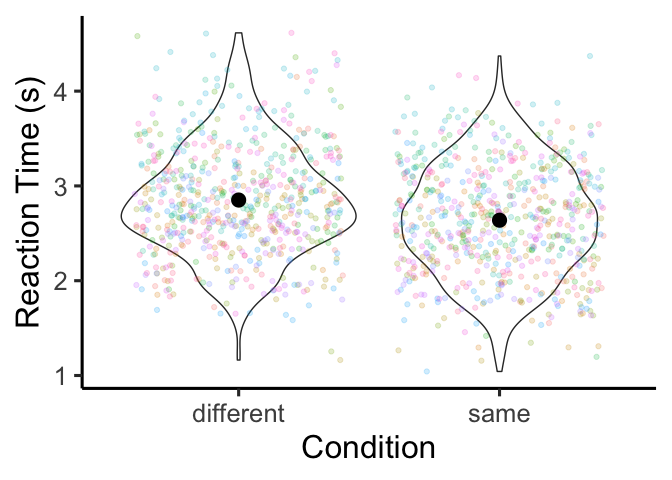
The means are pretty close to each other, but it looks like we might
have the effect we observed. To find out for sure, let’s run a
regression!
1
2
| m <- lm(RT ~ condition, df)
summary(m)
|
1
2
3
4
5
6
7
8
9
10
11
12
13
14
15
16
17
18
| ##
## Call:
## lm(formula = RT ~ condition, data = df)
##
## Residuals:
## Min 1Q Median 3Q Max
## -1.68792 -0.38280 -0.02851 0.39654 1.76337
##
## Coefficients:
## Estimate Std. Error t value Pr(>|t|)
## (Intercept) 2.85118 0.02291 124.428 < 2e-16 ***
## conditionsame -0.21303 0.03241 -6.574 7.19e-11 ***
## ---
## Signif. codes: 0 '***' 0.001 '**' 0.01 '*' 0.05 '.' 0.1 ' ' 1
##
## Residual standard error: 0.5729 on 1248 degrees of freedom
## Multiple R-squared: 0.03347, Adjusted R-squared: 0.03269
## F-statistic: 43.22 on 1 and 1248 DF, p-value: 7.187e-11
|
Based on the number of stars in this output, it looks like we have a
significant effect! But what exactly is significant? More
specifically, what do these coefficients actually mean? The answer
actually depends on how the contrasts over your variables are coded.
Dummy coding
By default, R uses a system of contrasts called dummy coding (or
contr.treatment). With dummy coding, we select one of the levels of
the variable as a reference level. For categorical variables, by
default, R assumes that you want use the earliest level of the
variable as the reference level (in our case, this is the ‘different’
condition). Then the Intercept is simply the mean RT for this
reference level. We can confirm this by calculating the mean manually:
1
2
| mean.different <- df %>% filter(condition=='different') %>% pull(RT) %>% mean
mean.different
|
Then, the coefficient conditionsame is the difference between the
means for our two conditions:
1
2
| mean.same <- df %>% filter(condition=='same') %>% pull(RT) %>% mean
mean.same - mean.different
|
Putting this together, our significant result is that reaction times
were slightly shorter for the “same” condition compared to the
“different” condition. What if we want the other way around? Easy- we
just set the desired reference level of the condition variable:
1
2
3
| df <- df %>% mutate(condition=factor(condition, levels=c('same', 'different')))
m <- lm(RT ~ condition, df)
summary(m)
|
1
2
3
4
5
6
7
8
9
10
11
12
13
14
15
16
17
18
| ##
## Call:
## lm(formula = RT ~ condition, data = df)
##
## Residuals:
## Min 1Q Median 3Q Max
## -1.68792 -0.38280 -0.02851 0.39654 1.76337
##
## Coefficients:
## Estimate Std. Error t value Pr(>|t|)
## (Intercept) 2.63815 0.02291 115.131 < 2e-16 ***
## conditiondifferent 0.21303 0.03241 6.574 7.19e-11 ***
## ---
## Signif. codes: 0 '***' 0.001 '**' 0.01 '*' 0.05 '.' 0.1 ' ' 1
##
## Residual standard error: 0.5729 on 1248 degrees of freedom
## Multiple R-squared: 0.03347, Adjusted R-squared: 0.03269
## F-statistic: 43.22 on 1 and 1248 DF, p-value: 7.187e-11
|
We can see that the Intercept now refers to the average RT in the
“same” condition, and the conditiondifferent coefficient now refers to
the difference between the same and different conditions. Notably, this
is the same value as before, but negative.
Sum-to-zero coding
Another popular way of coding regression coefficients is to use
sum-to-zero or effects coding (or contr.sum), which is popular in
psychology because it produces orthogonal (read: independent) contrasts
similar to an ANOVA. There are a couple different ways to change the
contrast coding in R, but I recommend doing it like so:
1
2
| m <- lm(RT ~ condition, df, contrasts=list(condition=contr.sum))
summary(m)
|
1
2
3
4
5
6
7
8
9
10
11
12
13
14
15
16
17
18
| ##
## Call:
## lm(formula = RT ~ condition, data = df, contrasts = list(condition = contr.sum))
##
## Residuals:
## Min 1Q Median 3Q Max
## -1.68792 -0.38280 -0.02851 0.39654 1.76337
##
## Coefficients:
## Estimate Std. Error t value Pr(>|t|)
## (Intercept) 2.7447 0.0162 169.393 < 2e-16 ***
## condition1 -0.1065 0.0162 -6.574 7.19e-11 ***
## ---
## Signif. codes: 0 '***' 0.001 '**' 0.01 '*' 0.05 '.' 0.1 ' ' 1
##
## Residual standard error: 0.5729 on 1248 degrees of freedom
## Multiple R-squared: 0.03347, Adjusted R-squared: 0.03269
## F-statistic: 43.22 on 1 and 1248 DF, p-value: 7.187e-11
|
Under sum-to-zero coding, the intercept is now the grand mean RT over
all of our data (more specifically, the mean of the mean RTs in each
condition), and the slope condition1 is the difference between this
grand mean and the mean RT of the “same” condition.
1
2
3
4
| mean.grand <- mean(c(mean.same, mean.different))
mean.grand
mean.same - mean.grand
|
1
2
| ## [1] 2.744662
## [1] -0.1065158
|
Thinking like a linear model
From the last two examples, hopefully it’s obvious that regression
coefficients are just differences between means. Specifically, our
regression model sees the world through a table like this:
That is, for each cell in this table, our model predicts a unique mean
reaction time. In this case, the predicted means are just the raw means
that we calculated above. But since this won’t work for every design,
I’m going to introduce you to the treasure that is emmeans. emmeans
stands for “expected marginal means” and does exactly that: it takes a
regression model and a set of independent variables, and tells you what
the model thinks the mean is for setting of the independent variables.
For example, let’s get the expected marginal means of RT by condition:
1
| emmeans(m, ~ condition)
|
1
2
3
4
5
| ## condition emmean SE df lower.CL upper.CL
## same 2.64 0.0229 1248 2.59 2.68
## different 2.85 0.0229 1248 2.81 2.90
##
## Confidence level used: 0.95
|
To reproduce the model’s coefficients, we can just pipe the output of
this statement into the contrast function. I don’t know why, but
emmeans names the contrasts differently from base R (helpful,
right?), such that contr.treatment is called trt.vs.ctrl, and
contr.sum is called eff:
1
2
3
4
5
6
7
| ## for dummy contrasts
emmeans(m, ~ condition) %>%
contrast('trt.vs.ctrl')
## for sum-to-zero contrasts
emmeans(m, ~ condition) %>%
contrast('eff')
|
1
2
3
4
5
6
7
8
| ## contrast estimate SE df t.ratio p.value
## different - same 0.213 0.0324 1248 6.574 <.0001
##
## contrast estimate SE df t.ratio p.value
## same effect -0.107 0.0162 1248 -6.574 <.0001
## different effect 0.107 0.0162 1248 6.574 <.0001
##
## P value adjustment: fdr method for 2 tests
|
Alternatively, we can put the contrasts directly into the left side of
the formula in the emmeans call to see the contrasts alongside the
means:
1
2
3
4
5
| ## for dummy contrasts
emmeans(m, trt.vs.ctrl ~ condition)
## for sum-to-zero contrasts
emmeans(m, eff ~ condition)
|
1
2
3
4
5
6
7
8
9
10
11
12
13
14
15
16
17
18
19
20
21
22
23
24
25
| ## $emmeans
## condition emmean SE df lower.CL upper.CL
## same 2.64 0.0229 1248 2.59 2.68
## different 2.85 0.0229 1248 2.81 2.90
##
## Confidence level used: 0.95
##
## $contrasts
## contrast estimate SE df t.ratio p.value
## different - same 0.213 0.0324 1248 6.574 <.0001
##
##
## $emmeans
## condition emmean SE df lower.CL upper.CL
## same 2.64 0.0229 1248 2.59 2.68
## different 2.85 0.0229 1248 2.81 2.90
##
## Confidence level used: 0.95
##
## $contrasts
## contrast estimate SE df t.ratio p.value
## same effect -0.107 0.0162 1248 -6.574 <.0001
## different effect 0.107 0.0162 1248 6.574 <.0001
##
## P value adjustment: fdr method for 2 tests
|
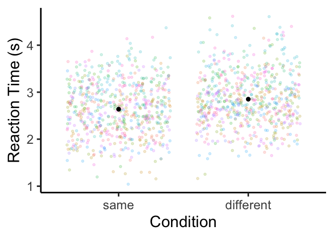
I’ll also note here that this is a fantastic way to get predicted
means/CIs to make a plot of your results, without having to calculate
anything manually (and yes, this even works for mixed-effect models and
repeated measures designs)! Let’s try it out:
1
2
3
4
5
6
| ggplot(df, aes(x=condition, y=RT)) +
geom_jitter(aes(color=participant), height=0, show.legend=F, alpha=0.2) +
geom_pointrange(aes(y=emmean, ymin=lower.CL, ymax=upper.CL),
data=as.data.frame(emmeans(m, ~ condition))) +
xlab('Condition') + ylab('Reaction Time (s)') +
theme_classic(base_size=24)
|
Regression with additive predictors
Until now, we’ve focused on interpreting regression coefficients when we
have just one predictor in our model. But things get a little messier
when we use two or more predictors. For example, perhaps we wanted to
know if the color of the stimulus also effects people’s reaction time in
the Stroop task. More specifically, we’d like to estimate a mean RT for
each cell of the following table:
|
|
condition
|
|
color
|
same, blue
|
different, blue
|
|
same, green
|
different,
green
|
|
same, red
|
different, red
|
There are two ways we could add this into our model. In the simplest
case, we might want to see if both (a) condition and (b) color
independently. That is, we force the effect of condition to be the
same across the different levels of color and vice versa. We can do
this using the + symbol in our regression formula:
1
2
| m <- lm(RT ~ condition + color, df)
summary(m)
|
1
2
3
4
5
6
7
8
9
10
11
12
13
14
15
16
17
18
19
20
| ##
## Call:
## lm(formula = RT ~ condition + color, data = df)
##
## Residuals:
## Min 1Q Median 3Q Max
## -1.64646 -0.38321 -0.03082 0.40313 1.73237
##
## Coefficients:
## Estimate Std. Error t value Pr(>|t|)
## (Intercept) 2.63205 0.03324 79.173 < 2e-16 ***
## conditiondifferent 0.21597 0.03240 6.666 3.93e-11 ***
## colorgreen -0.03829 0.04012 -0.954 0.340
## colorred 0.04998 0.03974 1.258 0.209
## ---
## Signif. codes: 0 '***' 0.001 '**' 0.01 '*' 0.05 '.' 0.1 ' ' 1
##
## Residual standard error: 0.5721 on 1246 degrees of freedom
## Multiple R-squared: 0.03742, Adjusted R-squared: 0.0351
## F-statistic: 16.14 on 3 and 1246 DF, p-value: 2.674e-10
|
It looks like we have a significant effect of condition, and no
significant effects of color. To replicate these coefficients, we can
use emmeans (the adjust='none' option is used to make sure the
p-values match what we get from lm):
1
2
| emmeans(m, ~ condition) %>% contrast('trt.vs.ctrl')
emmeans(m, ~ color) %>% contrast('trt.vs.ctrl', adjust='none')
|
1
2
3
4
5
6
7
8
9
| ## contrast estimate SE df t.ratio p.value
## different - same 0.216 0.0324 1246 6.666 <.0001
##
## Results are averaged over the levels of: color
## contrast estimate SE df t.ratio p.value
## green - blue -0.0383 0.0401 1246 -0.954 0.3400
## red - blue 0.0500 0.0397 1246 1.258 0.2087
##
## Results are averaged over the levels of: condition
|
We can see that the Intercept is our estimate of the mean RT for
trials in the “same” condition with a blue stimulus, the
conditiondifferent coefficient is the average increase in RT for the
different condition over the three colors, and the two color
coefficients are the difference between mean RT in the red/green and
blue colors, averaging over the two conditions. To confirm that our
model actually treats the effects of condition and color independently,
we can compute contrasts of one variable over the levels of the other
variable:
1
2
| emmeans(m, ~condition|color) %>% contrast('trt.vs.ctrl')
emmeans(m, ~color|condition) %>% contrast('trt.vs.ctrl', adjust='none')
|
1
2
3
4
5
6
7
8
9
10
11
12
13
14
15
16
17
18
19
20
21
| ## color = blue:
## contrast estimate SE df t.ratio p.value
## different - same 0.216 0.0324 1246 6.666 <.0001
##
## color = green:
## contrast estimate SE df t.ratio p.value
## different - same 0.216 0.0324 1246 6.666 <.0001
##
## color = red:
## contrast estimate SE df t.ratio p.value
## different - same 0.216 0.0324 1246 6.666 <.0001
##
## condition = same:
## contrast estimate SE df t.ratio p.value
## green - blue -0.0383 0.0401 1246 -0.954 0.3400
## red - blue 0.0500 0.0397 1246 1.258 0.2087
##
## condition = different:
## contrast estimate SE df t.ratio p.value
## green - blue -0.0383 0.0401 1246 -0.954 0.3400
## red - blue 0.0500 0.0397 1246 1.258 0.2087
|
Since the contrasts look the same over each level of the variable, we
can be sure that our model does not allow condition and color to
interact. If we want to use different contrast coding for this model,
the coefficients are just as interpretable. For example, we can estimate
the same model with sum-to-zero coefficients:
1
2
| m <- lm(RT ~ condition + color, df, contrasts=list(condition='contr.sum', color='contr.sum'))
summary(m)
|
1
2
3
4
5
6
7
8
9
10
11
12
13
14
15
16
17
18
19
20
21
| ##
## Call:
## lm(formula = RT ~ condition + color, data = df, contrasts = list(condition = "contr.sum",
## color = "contr.sum"))
##
## Residuals:
## Min 1Q Median 3Q Max
## -1.64646 -0.38321 -0.03082 0.40313 1.73237
##
## Coefficients:
## Estimate Std. Error t value Pr(>|t|)
## (Intercept) 2.743929 0.016195 169.428 < 2e-16 ***
## condition1 -0.107984 0.016198 -6.666 3.93e-11 ***
## color1 -0.003897 0.023196 -0.168 0.8666
## color2 -0.042191 0.022882 -1.844 0.0654 .
## ---
## Signif. codes: 0 '***' 0.001 '**' 0.01 '*' 0.05 '.' 0.1 ' ' 1
##
## Residual standard error: 0.5721 on 1246 degrees of freedom
## Multiple R-squared: 0.03742, Adjusted R-squared: 0.0351
## F-statistic: 16.14 on 3 and 1246 DF, p-value: 2.674e-10
|
The coefficients can be interpreted in the same way as sum-to-zero
contrasts with only one variable: the intercept corresponds to our
estimate of the grand mean, the coefficient for condition is the
difference between the grand mean and the same condition, and the color
coefficients are the difference between the grand mean and the red/green
colors:
1
2
| emmeans(m, ~ condition) %>% contrast('eff')
emmeans(m, ~ color) %>% contrast('eff', adjust='none')
|
1
2
3
4
5
6
7
8
9
10
11
12
| ## contrast estimate SE df t.ratio p.value
## same effect -0.108 0.0162 1246 -6.666 <.0001
## different effect 0.108 0.0162 1246 6.666 <.0001
##
## Results are averaged over the levels of: color
## P value adjustment: fdr method for 2 tests
## contrast estimate SE df t.ratio p.value
## blue effect -0.0039 0.0232 1246 -0.168 0.8666
## green effect -0.0422 0.0229 1246 -1.844 0.0654
## red effect 0.0461 0.0227 1246 2.034 0.0422
##
## Results are averaged over the levels of: condition
|
Of course, we can always mix + match the two coding systems together if
we so choose:
1
2
| m <- lm(RT ~ condition + color, df, contrasts=list(color='contr.sum'))
summary(m)
|
1
2
3
4
5
6
7
8
9
10
11
12
13
14
15
16
17
18
19
20
| ##
## Call:
## lm(formula = RT ~ condition + color, data = df, contrasts = list(color = "contr.sum"))
##
## Residuals:
## Min 1Q Median 3Q Max
## -1.64646 -0.38321 -0.03082 0.40313 1.73237
##
## Coefficients:
## Estimate Std. Error t value Pr(>|t|)
## (Intercept) 2.635945 0.022922 114.999 < 2e-16 ***
## conditiondifferent 0.215969 0.032396 6.666 3.93e-11 ***
## color1 -0.003897 0.023196 -0.168 0.8666
## color2 -0.042191 0.022882 -1.844 0.0654 .
## ---
## Signif. codes: 0 '***' 0.001 '**' 0.01 '*' 0.05 '.' 0.1 ' ' 1
##
## Residual standard error: 0.5721 on 1246 degrees of freedom
## Multiple R-squared: 0.03742, Adjusted R-squared: 0.0351
## F-statistic: 16.14 on 3 and 1246 DF, p-value: 2.674e-10
|
As an exercise, see if you can figure out where these numbers come from
(hint: look up!).
Regression with interacting predictors
While the additive model is nice and easy to interpret, it’s not always
the case that the effect of one variable will be the same across the
domain of another variable. To relax this assumption, we can fit a
multiplicative model that includes interaction terms:
1
2
| m <- lm(RT ~ condition * color, df)
summary(m)
|
1
2
3
4
5
6
7
8
9
10
11
12
13
14
15
16
17
18
19
20
21
22
| ##
## Call:
## lm(formula = RT ~ condition * color, data = df)
##
## Residuals:
## Min 1Q Median 3Q Max
## -1.67893 -0.37766 -0.03314 0.40012 1.74843
##
## Coefficients:
## Estimate Std. Error t value Pr(>|t|)
## (Intercept) 2.63452 0.04128 63.820 < 2e-16 ***
## conditiondifferent 0.21117 0.05751 3.672 0.000251 ***
## colorgreen -0.07548 0.05765 -1.309 0.190709
## colorred 0.07582 0.05586 1.357 0.174949
## conditiondifferent:colorgreen 0.07197 0.08026 0.897 0.370050
## conditiondifferent:colorred -0.05540 0.07950 -0.697 0.486034
## ---
## Signif. codes: 0 '***' 0.001 '**' 0.01 '*' 0.05 '.' 0.1 ' ' 1
##
## Residual standard error: 0.572 on 1244 degrees of freedom
## Multiple R-squared: 0.03946, Adjusted R-squared: 0.0356
## F-statistic: 10.22 on 5 and 1244 DF, p-value: 1.293e-09
|
You can see that now we have two more interaction coefficients. Under
dummy coding, the presence of these interaction coefficients changes how
the above coefficients are interpreted: now, each coefficient is
conditional with respect to the reference level of each variable. The
Intercept is still the mean RT for trials in the “same” condition
with a blue stimulus. But, whereas the conditiondifferent used to tell
us the average difference between same/different trials over the three
colors, now it only tells us that difference for the blue trials. We
call this a “simple effect” since its interpretation is more simple than
that of a “main effect” which we’ll talk about soon. In emmeans, we
can get this contrast for the blue trials only using the at argument:
1
2
| emmeans(m, ~ condition | color, at=list(color=c('blue'))) %>%
contrast('trt.vs.ctrl')
|
1
2
3
| ## color = blue:
## contrast estimate SE df t.ratio p.value
## different - same 0.211 0.0575 1244 3.672 0.0003
|
The colorgreen and colorred coefficients have also changed: now they
are the difference between the blue and red/green colors within the
“same” condition:
1
2
| emmeans(m, ~ color | condition, at=list(condition=c('same'))) %>%
contrast('trt.vs.ctrl', adjust='none')
|
1
2
3
4
| ## condition = same:
## contrast estimate SE df t.ratio p.value
## green - blue -0.0755 0.0577 1244 -1.309 0.1907
## red - blue 0.0758 0.0559 1244 1.357 0.1749
|
Finally, we have the two interaction terms. There are two equally good
ways of thinking about them. On one hand, they are the difference in the
same/different Stroop effect between the red/green and blue colored
trials:
1
2
3
| emmeans(m, ~ condition | color) %>%
contrast('trt.vs.ctrl') %>%
contrast(method='trt.vs.ctrl', by='contrast', adjust='none')
|
1
2
3
4
| ## contrast = different - same:
## contrast1 estimate SE df t.ratio p.value
## green - blue 0.0720 0.0803 1244 0.897 0.3700
## red - blue -0.0554 0.0795 1244 -0.697 0.4860
|
This tells us that the Stroop effect was larger for green than for blue
stimuli, and larger for blue than for red stimuli (though none of these
differences were significant). But another way of looking at it is that
they describe the difference in the differences between stimulus colors
across the same/different conditions:
1
2
3
| emmeans(m, ~ color | condition) %>%
contrast('trt.vs.ctrl') %>%
contrast(method='trt.vs.ctrl', by='contrast', adjust='none')
|
1
2
3
4
5
6
7
| ## contrast = green - blue:
## contrast1 estimate SE df t.ratio p.value
## different - same 0.0720 0.0803 1244 0.897 0.3700
##
## contrast = red - blue:
## contrast1 estimate SE df t.ratio p.value
## different - same -0.0554 0.0795 1244 -0.697 0.4860
|
This perspective tells us that the difference between RTs following
green and blue stimuli in the “different” condition is larger than in
the “same” condition, and that the difference between RTs following red
and blue stimuli in the “different” condition is smaller than in the
“same” condition. In this case the first interpretation is more natural,
but mathematically both interpretations are equivalent, so feel free to
take whichever interpretation seems more natural.
If you’re used to running ANOVAs, then it might seem that the approach
of looking at effects of one variable conditional on another is more
complicated than it needs to be. What you really want to know is, on
average, what does effect does each predictor have on the outcome
variable- you want a main effect. We can get main effects by switching
from dummy contrasts to sum-to-zero contrasts:
1
2
| m <- lm(RT ~ condition * color, df, contrasts=list(condition='contr.sum', color='contr.sum'))
summary(m)
|
1
2
3
4
5
6
7
8
9
10
11
12
13
14
15
16
17
18
19
20
21
22
23
| ##
## Call:
## lm(formula = RT ~ condition * color, data = df, contrasts = list(condition = "contr.sum",
## color = "contr.sum"))
##
## Residuals:
## Min 1Q Median 3Q Max
## -1.67893 -0.37766 -0.03314 0.40012 1.74843
##
## Coefficients:
## Estimate Std. Error t value Pr(>|t|)
## (Intercept) 2.742980 0.016206 169.258 < 2e-16 ***
## condition1 -0.108349 0.016206 -6.686 3.46e-11 ***
## color1 -0.002875 0.023201 -0.124 0.9014
## color2 -0.042367 0.022887 -1.851 0.0644 .
## condition1:color1 0.002762 0.023201 0.119 0.9052
## condition1:color2 -0.033224 0.022887 -1.452 0.1469
## ---
## Signif. codes: 0 '***' 0.001 '**' 0.01 '*' 0.05 '.' 0.1 ' ' 1
##
## Residual standard error: 0.572 on 1244 degrees of freedom
## Multiple R-squared: 0.03946, Adjusted R-squared: 0.0356
## F-statistic: 10.22 on 5 and 1244 DF, p-value: 1.293e-09
|
Now we can go back to treating each coefficient in isolation: the
Intercept is the grand mean, the condition1 coefficient tells us the
average difference between the same condition and the grand mean over
all stimulus colors, the color1 and color2 are the average
differences between the blue/green colors and the grand mean over both
conditions, and finally the interaction terms are the difference in the
difference in the same condition and the grand mean between the
blue/green colors and the grand mean. Even though this sounds like a
mouthful, sum-to-zero contrasts have the advantage that each coefficient
is independent of the others.
Continuous variables
We’ve been through interpreting the null regression model, interpreting
single-variable regression models, and interpreting regression models
with more than one variable. What could possibly be left? Well, if you
remember back to when we simulated this data, we also simulated the
saturation level of the stimulus color (ranging from 0 to 100%). This is
a continuous variable, which has some quirks of its own in terms of
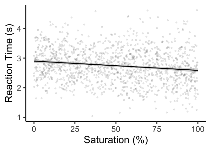
interpreting regression coefficients. Let’s start by forgetting about
the Stroop effect, and just looking at whether saturation influences
reaction time during the Stroop task:
1
2
3
4
5
| ggplot(df, aes(x=saturation, y=RT)) +
geom_point(alpha=.1) +
geom_smooth(color='black', method='lm') +
xlab('Saturation (%)') + ylab('Reaction Time (s)') +
theme_classic(base_size=24)
|
To β or not to β?
It turns out that there are a few different ways to code this very same
regression. Let’s start by running a regression using R’s default
settings:
1
2
| m <- lm(RT ~ saturation, df)
summary(m)
|
1
2
3
4
5
6
7
8
9
10
11
12
13
14
15
16
17
18
| ##
## Call:
## lm(formula = RT ~ saturation, data = df)
##
## Residuals:
## Min 1Q Median 3Q Max
## -1.7448 -0.3810 -0.0215 0.3804 2.0264
##
## Coefficients:
## Estimate Std. Error t value Pr(>|t|)
## (Intercept) 2.8988005 0.0318273 91.079 < 2e-16 ***
## saturation -0.0031243 0.0005544 -5.636 2.16e-08 ***
## ---
## Signif. codes: 0 '***' 0.001 '**' 0.01 '*' 0.05 '.' 0.1 ' ' 1
##
## Residual standard error: 0.5754 on 1248 degrees of freedom
## Multiple R-squared: 0.02482, Adjusted R-squared: 0.02404
## F-statistic: 31.76 on 1 and 1248 DF, p-value: 2.155e-08
|
With this default setting, we interpret the coefficients similarly to
dummy-coded categorical variables. That is, the Intercept is the mean
RT when saturation is zero, and the saturation coefficient is the
mean increase/decrease in RTs when saturation is increased by 1. Since
our saturation variable is in percentage units, this is the increase
in RT with a 1% increase in saturation. If you want to make your
Intercept more interpretable, you can standardize the predictor
variable saturation by subtracting the mean and dividing by the
standard deviation (done by the scale function):
1
2
3
| df$saturation.std <- scale(df$saturation)
m <- lm(RT ~ saturation.std, df)
summary(m)
|
1
2
3
4
5
6
7
8
9
10
11
12
13
14
15
16
17
18
| ##
## Call:
## lm(formula = RT ~ saturation.std, data = df)
##
## Residuals:
## Min 1Q Median 3Q Max
## -1.7448 -0.3810 -0.0215 0.3804 2.0264
##
## Coefficients:
## Estimate Std. Error t value Pr(>|t|)
## (Intercept) 2.74466 0.01628 168.640 < 2e-16 ***
## saturation.std -0.09176 0.01628 -5.636 2.16e-08 ***
## ---
## Signif. codes: 0 '***' 0.001 '**' 0.01 '*' 0.05 '.' 0.1 ' ' 1
##
## Residual standard error: 0.5754 on 1248 degrees of freedom
## Multiple R-squared: 0.02482, Adjusted R-squared: 0.02404
## F-statistic: 31.76 on 1 and 1248 DF, p-value: 2.155e-08
|
Though the Intercept is still the mean RT when saturation.std is
zero, this has a different interpretation before. Since saturation.std
is standardized, it is centered at zero and has a standard deviation of
- So, the
Intercept is the mean RT at the mean value of saturation,
and the coefficient saturation.std is the mean increase in RT with a
standard deviation increase in saturation. In cases where the
predictor variable has a meaningless scale (like a Likert scale), this
coefficient can be more interpretable than the default coefficient.
Finally, in addition to standardizing the predictor variable
saturation, we can also standardize the outcome variable RT:
1
2
3
| df$RT.std <- scale(df$RT)
m <- lm(RT.std ~ saturation.std, df)
summary(m)
|
1
2
3
4
5
6
7
8
9
10
11
12
13
14
15
16
17
18
| ##
## Call:
## lm(formula = RT.std ~ saturation.std, data = df)
##
## Residuals:
## Min 1Q Median 3Q Max
## -2.9956 -0.6541 -0.0369 0.6531 3.4791
##
## Coefficients:
## Estimate Std. Error t value Pr(>|t|)
## (Intercept) 9.950e-17 2.794e-02 0.000 1
## saturation.std -1.575e-01 2.795e-02 -5.636 2.16e-08 ***
## ---
## Signif. codes: 0 '***' 0.001 '**' 0.01 '*' 0.05 '.' 0.1 ' ' 1
##
## Residual standard error: 0.9879 on 1248 degrees of freedom
## Multiple R-squared: 0.02482, Adjusted R-squared: 0.02404
## F-statistic: 31.76 on 1 and 1248 DF, p-value: 2.155e-08
|
Now, the Intercept is extremely close to zero (representing the mean
standardized RT at the mean saturation), and the coefficient
saturation.std is the standardi deviation increase in RT given a
standard deviation increase in saturation: in other words, it’s a
correlation!
1
| cor.test(df$RT.std, df$saturation.std)
|
1
2
3
4
5
6
7
8
9
10
11
| ##
## Pearson's product-moment correlation
##
## data: df$RT.std and df$saturation.std
## t = -5.6355, df = 1248, p-value = 2.155e-08
## alternative hypothesis: true correlation is not equal to 0
## 95 percent confidence interval:
## -0.2111345 -0.1029865
## sample estimates:
## cor
## -0.1575328
|
You can also run the regression with standardized RTs, but not
standardized saturation values. As an exercise, try interpreting these
(standardized) coefficients:
1
2
| m <- lm(RT.std ~ saturation, df)
summary(m)
|
1
2
3
4
5
6
7
8
9
10
11
12
13
14
15
16
17
18
| ##
## Call:
## lm(formula = RT.std ~ saturation, data = df)
##
## Residuals:
## Min 1Q Median 3Q Max
## -2.9956 -0.6541 -0.0369 0.6531 3.4791
##
## Coefficients:
## Estimate Std. Error t value Pr(>|t|)
## (Intercept) 0.2646347 0.0546429 4.843 1.44e-06 ***
## saturation -0.0053641 0.0009518 -5.636 2.16e-08 ***
## ---
## Signif. codes: 0 '***' 0.001 '**' 0.01 '*' 0.05 '.' 0.1 ' ' 1
##
## Residual standard error: 0.9879 on 1248 degrees of freedom
## Multiple R-squared: 0.02482, Adjusted R-squared: 0.02404
## F-statistic: 31.76 on 1 and 1248 DF, p-value: 2.155e-08
|
If you have been paying attention, you’ll have noticed that the
significance of the saturation coefficient was exactly the same
between the four versions of the model. Ultimately, the choice to
standardize or not to standardize is totally up to you and your
preferences.
Combining continuous & categorical
We found that saturation decreased RTs in the Stroop task on average.
Could this effect differ depending on whether the color of the stimulus
matched the text? First, let’s make a plot:
1
2
3
4
5
| ggplot(df, aes(x=saturation, y=RT, color=condition)) +
geom_point(alpha=.1) +
geom_smooth(method='lm') +
xlab('Saturation (%)') + ylab('Reaction Time (s)') +
theme_classic()
|
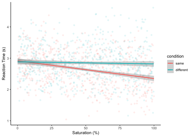
It looks like RTs only decrease with saturation when the color is the
same as the text. To confirm, let’s run a (multiplicative) regression:
1
2
| m <- lm(RT ~ condition * saturation, df)
summary(m)
|
1
2
3
4
5
6
7
8
9
10
11
12
13
14
15
16
17
18
19
20
| ##
## Call:
## lm(formula = RT ~ condition * saturation, data = df)
##
## Residuals:
## Min 1Q Median 3Q Max
## -1.67095 -0.39058 -0.03076 0.37961 1.79690
##
## Coefficients:
## Estimate Std. Error t value Pr(>|t|)
## (Intercept) 2.9146551 0.0436345 66.797 < 2e-16 ***
## conditiondifferent -0.0300392 0.0620630 -0.484 0.628
## saturation -0.0056408 0.0007634 -7.389 2.70e-13 ***
## conditiondifferent:saturation 0.0049673 0.0010811 4.595 4.77e-06 ***
## ---
## Signif. codes: 0 '***' 0.001 '**' 0.01 '*' 0.05 '.' 0.1 ' ' 1
##
## Residual standard error: 0.561 on 1246 degrees of freedom
## Multiple R-squared: 0.07459, Adjusted R-squared: 0.07236
## F-statistic: 33.48 on 3 and 1246 DF, p-value: < 2.2e-16
|
Just like before, the Intercept is the mean RT when condition is
at its reference level (“same”), and when saturation is at zero,
conditiondifferent tells us the mean Stroop effect when saturation
is at zero, and saturation tells us the increase in RT with a 1%
increase in saturation in the “same” condition:
1
2
3
4
5
6
7
8
9
10
| ## Intercept
emmeans(m, ~condition, at=list(condition='same', saturation=0))
## conditiondifferent
emmeans(m, ~condition, at=list(saturation=0)) %>%
contrast('trt.vs.ctrl')
## saturation
emmeans(m, ~saturation, at=list(saturation=0:1, condition='same')) %>%
contrast('trt.vs.ctrl')
|
1
2
3
4
5
6
7
8
9
| ## condition emmean SE df lower.CL upper.CL
## same 2.91 0.0436 1246 2.83 3
##
## Confidence level used: 0.95
## contrast estimate SE df t.ratio p.value
## different - same -0.03 0.0621 1246 -0.484 0.6285
##
## contrast estimate SE df t.ratio p.value
## 1 - 0 -0.00564 0.000763 1246 -7.389 <.0001
|
As with the interaction between condition and color, there are two
different ways we can choose to interpret the interaction coefficient.
First, we could say that it is the difference in size of the Stroop
effect between when saturation = 1% and when saturation = 0%. But
it’s equally accurate to say that it represents the difference in the
effect of saturation between the “same” and “different” conditions:
1
2
3
4
5
6
7
| emmeans(m, ~ saturation | condition, at=list(saturation=0:1)) %>%
contrast('trt.vs.ctrl') %>%
contrast(method='trt.vs.ctrl', by='contrast', adjust='none')
emmeans(m, ~ condition | saturation, at=list(saturation=0:1)) %>%
contrast('trt.vs.ctrl') %>%
contrast(method='trt.vs.ctrl', by='contrast', adjust='none')
|
1
2
3
4
5
6
7
| ## contrast = 1 - 0:
## contrast1 estimate SE df t.ratio p.value
## different - same 0.00497 0.00108 1246 4.595 <.0001
##
## contrast = different - same:
## contrast1 estimate SE df t.ratio p.value
## 1 - 0 0.00497 0.00108 1246 4.595 <.0001
|
As an exercise, try repeating this regression with sum-to-zero contrasts
and interpreting those coefficients!
Link functions and you
There’s one more case where you might be having trouble interpreting
regression coefficients: when using a family other than the default
Gaussian, particilarly families with non-identity link functions. In
logistic regression, for example, we predict a binary outcome with a
linear regression on the logit scale (from − ∞ to ∞), which gets
pumped through the inverse logit function to yield probabilities (from 0
to 1). This transformation can sometimes make interpreting the
coefficients difficult. As an example, let’s try looking at whether, in
addition to being slower, people also make more mistakes when the
stimulus text and color are different. First, as always, let’s check out
a plot:
1
2
3
4
5
| ggplot(df, aes(x=condition, y=correct)) +
geom_jitter(alpha=.1, height=0) +
stat_summary(fun.data=mean_cl_normal) +
xlab('Condition') + ylab('Probability of Correct Response') +
theme_classic()
|
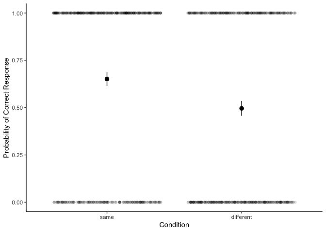
It appears as if people perform above chance in the “same” condition,
but not the “different” condition. To confirm, let’s look at the
underlying model:
1
2
| m <- glm(correct ~ condition, df, family='binomial')
summary(m)
|
1
2
3
4
5
6
7
8
9
10
11
12
13
14
15
16
17
18
19
20
21
22
| ##
## Call:
## glm(formula = correct ~ condition, family = "binomial", data = df)
##
## Deviance Residuals:
## Min 1Q Median 3Q Max
## -1.4514 -1.1706 0.9262 0.9262 1.1842
##
## Coefficients:
## Estimate Std. Error z value Pr(>|z|)
## (Intercept) 0.62432 0.08393 7.439 1.02e-13 ***
## conditiondifferent -0.64032 0.11595 -5.522 3.35e-08 ***
## ---
## Signif. codes: 0 '***' 0.001 '**' 0.01 '*' 0.05 '.' 0.1 ' ' 1
##
## (Dispersion parameter for binomial family taken to be 1)
##
## Null deviance: 1705.7 on 1249 degrees of freedom
## Residual deviance: 1674.8 on 1248 degrees of freedom
## AIC: 1678.8
##
## Number of Fisher Scoring iterations: 4
|
We can see that both the Intercept and the conditiondifferent
coefficients are significant. But what do they mean? Similarly to
before, the Intercept is the mean X for the “same” condition, and
conditiondifferent is the mean change in X between the “same” and
“different” conditions. To find out what X exactly is, let’s consult
emmeans:
1
| emmeans(m, ~ condition)
|
1
2
3
4
5
6
| ## condition emmean SE df asymp.LCL asymp.UCL
## same 0.624 0.0839 Inf 0.460 0.789
## different -0.016 0.0800 Inf -0.173 0.141
##
## Results are given on the logit (not the response) scale.
## Confidence level used: 0.95
|
emmeans tells us that our estimates are on the logit scale, not the
response scale. Although we could transform these manually back to
probabilities using the function plogis, emmeans can do it for you:
1
| emmeans(m, ~ condition, type='response')
|
1
2
3
4
5
6
| ## condition prob SE df asymp.LCL asymp.UCL
## same 0.651 0.0191 Inf 0.613 0.688
## different 0.496 0.0200 Inf 0.457 0.535
##
## Confidence level used: 0.95
## Intervals are back-transformed from the logit scale
|
Now we can see that the probability of responding correctly is 65% in
the same condition and 50% in the different condition. Are these two
probabilities different? Let’s find out:
1
| emmeans(m, ~ condition, type='response') %>% contrast('trt.vs.ctrl')
|
1
2
3
4
| ## contrast odds.ratio SE df null z.ratio p.value
## different / same 0.527 0.0611 Inf 1 -5.522 <.0001
##
## Tests are performed on the log odds ratio scale
|
Whoah- what’s going on there? Instead of differences in probabilities,
emmeans is giving us something called an odds ratio. What’s that? Well
an odds is the proportion between something happening and not
happening. We can calculate these manually:
1
2
3
4
5
6
7
8
| p.same <- as.data.frame(emmeans(m, ~ condition, type='response'))$prob[1]
p.diff <- as.data.frame(emmeans(m, ~ condition, type='response'))$prob[2]
odds.same <- p.same / (1 - p.same)
odds.diff <- p.diff / (1 - p.diff)
odds.same
odds.diff
|
1
2
| ## [1] 1.866972
## [1] 0.984127
|
We can see that in the “same” condition, participants were 1.9 times
more likely to make a correct response compared to an incorrect
response. In the “different” condition, people were about as likely to
be correct as they were incorrrect. The odds ratio, not surprisingly, is
the ratio between these two odds:
1
2
| odds.ratio <- odds.diff / odds.same
odds.ratio
|
So we can piece all this back together to say that the odds of being
correct were about half as large in the different condition than in the
same condition. Why does emmeans give us this weird number? Well, this
is just what logistic regression tests for. Specifically, the logit
scale is also known as the log odds scale, which means that our
coefficients are on the scale of log odds. To convert our coefficients
to the odds scale, then, we can just exponentiate:
1
2
3
4
| exp(coef(m)) ## get the coefficients on the odds scale
## get the odds with CIs with emmeans
emmeans(m, ~condition, tran='log', type='response')
|
1
2
3
4
5
6
7
8
| ## (Intercept) conditiondifferent
## 1.8669725 0.5271245
## condition prob SE df asymp.LCL asymp.UCL
## same 1.867 0.1567 Inf 1.584 2.20
## different 0.984 0.0787 Inf 0.841 1.15
##
## Confidence level used: 0.95
## Intervals are back-transformed from the log scale
|
If odds ratios aren’t very intuitive for you, you are in good company.
Some have argued
that it’s not only fine, but it’s preferable to use standard linear
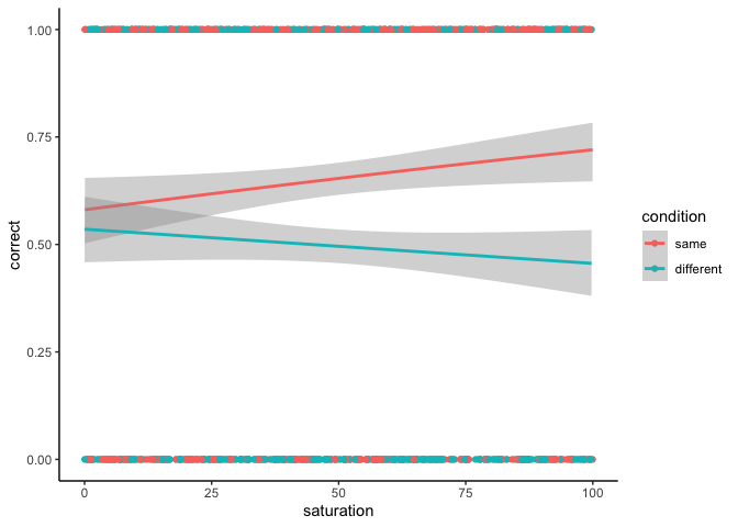
regression for estimating differences in probabilities. But if you’re
looking for more practice, as a parting exercise, try running this
logistic regression with condition and saturation as predictors! The
coefficients might take some work to interpret, but the basic logic is
exactly the same.
1
2
3
4
| ggplot(df, aes(x=saturation, y=correct, color=condition)) +
geom_point() +
geom_smooth(method='glm', method.args=list(family='binomial')) +
theme_classic()
|
Wrapping up
If you made it this far, congrats! We covered a lot in this workshop,
including how to interpret linear regression coefficients with zero-two
categorical variables, with standardized and unstandardized continuous
variables, and with non-trivial link functions (using the example of
logistic regression). In fact, we covered so much, that there’s not much
more to know here! With a little imagination, you can use the same logic
to interpret coefficients for models with 3+ way interactions, models
with random effects, and models with different link functions and
distribution families.