
Quick and Easy EEG Preprocessing in EEGLAB/ERPLAB

Why preprocess data?
EEG data is a continuous signal that only measures a difference of potentials at electrode locations. To make sense of the data we need to:
- extract meaningful measures from it, e.g., brain oscillations
- compare brain data in different conditions
- assess reliable changes due to external stimuli (event-related potentials)
In order to accomplish these goals, we need to transform (preprocess) the noisy data:
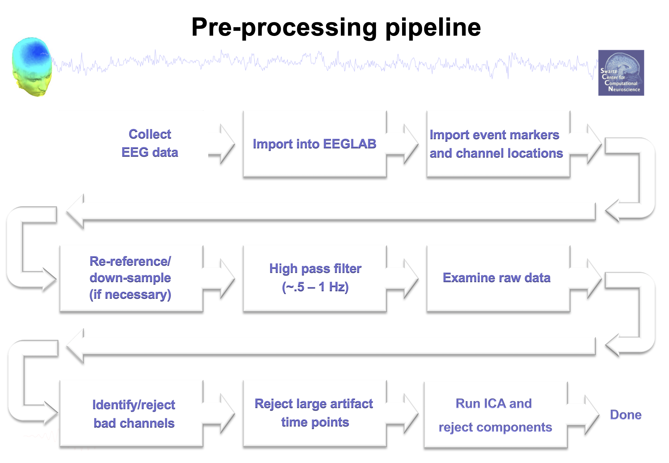
****General EEG Data Pre-processing Pipeline (from eeglab wiki)****
This tutorial
There are many ways to pre-process EEG data. In this example, we will use EEGLAB & ERPLAB functions.
Materials are adapted from ERP-CORE, a free online resource with experiment control scripts, data, and data analysis scripts assembled by the developers of ERPLAB.
In this simplified demo, we are using data from their P3 oddball paradigm:
If you have MATLAB, feel free to download these files so that you can explore the data in some of the demos! This is optional: you should be able to follow along either way.
Pre-processing pipeline:
- Configuring data: downsample, rereference, load channel locations
- Filter
- 0.1 Hz high pass
- ICA
- subtract obvious artifact components from data
- Epoch and bin trials
- cut continuous EEG recording into trial-sized chunks (epoch)
- sort trials into experiment conditions (bin)
- Artifact detection
- moving window peak-to-peak with subject specific thresholds and window sizes
- tags trials containing blinks, skin potentials, electrode noise that were not corrected by ICA
- Compute individual subject ERPs
- Grand Averaging (not covered)
Step 1: Configuring data
1
2
3
4
5
6
7
8
9
10
11
12
13
14
15
16
17
18
19
20
21
22
23
24
25
26
27
28
29
30
31
32
33
34
35
36
37
38
39
40
41
42
43
44
45
46
47
48
49
%Operates on individual subject data

%loads the raw continuous EEG data in .set EEGLAB file format,
%downsamples the data to 256 Hz to speed data processing time,
%references to the average of P9 and P10 (mastoid adjacent channels),
%creates bipolar HEOG and VEOG channels, adds channel location information, removes the DC offsets, and applies a high-pass filter.

close all; clearvars;

%Location of the main study directory
DIR = '/Users/audreyliu/Library/CloudStorage/Box-Box/methods_jc_eeg/P3/data'

%Location of the folder that contains this script and any associated processing files
Current_File_Path = '/Users/audreyliu/Library/CloudStorage/Box-Box/methods_jc_eeg/P3/EEG_ERP_Processing'

%List of subjects to process, based on the name of the folder that contains that subject's data
SUB = {'1', '2', '3'};

%***********************************************************************************************************************************************

%Loop through each subject listed in SUB
for i = 1:length(SUB)

	%Open EEGLAB and ERPLAB Toolboxes
	[ALLEEG EEG CURRENTSET ALLCOM] = eeglab;

	%Define subject path based on study directory and subject ID of current subject
	Subject_Path = [DIR filesep SUB{i} filesep];

	%Load the raw continuous EEG data file in .set EEGLAB file format
	EEG = pop_loadset( 'filename', [SUB{i} '_P3.set'], 'filepath', Subject_Path);
	%save new file after each step
	[ALLEEG EEG CURRENTSET] = pop_newset(ALLEEG, EEG, 1, 'setname', [SUB{i} '_P3'], 'gui', 'off');

	%Downsample from the recorded sampling rate of 1024 Hz to 256 Hz to speed data processing (automatically applies the appropriate low-pass anti-aliasing filter)
	EEG = pop_resample( EEG, 256);
	[ALLEEG EEG CURRENTSET] = pop_newset(ALLEEG, EEG, 2,'setname',[SUB{i} '_P3_ds'],'savenew',[Subject_Path SUB{i} '_P3_shifted_ds.set'] ,'gui','off');

	%Rereference to the average of P9 and P10; create a bipolar HEOG channel (HEOG_left minus HEOG_right) and a bipolar VEOG channel (VEOG_lower minus FP2)
	EEG = pop_eegchanoperator( EEG, [Current_File_Path filesep 'Rereference_Add_Uncorrected_Bipolars_P3.txt']);

	%Add channel location information corresponding to the 3-D coordinates of the electrodes based on 10-10 International System site locations
	EEG = pop_chanedit(EEG, 'lookup',[Current_File_Path filesep 'standard-10-5-cap385.elp']);
	[ALLEEG EEG CURRENTSET] = pop_newset(ALLEEG, EEG, 3, 'setname', [SUB{i} '_P3_ds_reref_ucbip'], 'savenew', [Subject_Path SUB{i} '_P3_shifted_ds_reref_ucbip.set'], 'gui', 'off');

%End subject loop
end

%***********************************************************************************************************************************************
Tip: It is helpful to save a new data file each time you do something to your data, so you can return to previous versions without rerunning your whole pipeline if something goes wrong. For low-tech version control, each time you do something new to the data set, append that step to the end of the file name: e.g. ‘1_P3.set’ becomes ‘1_P2_ds.set’ after downsampling (ds).
Now that we have given eeglab some basic information about the dataset (channel locations and reference voltage), let’s plot the data to see what we have!
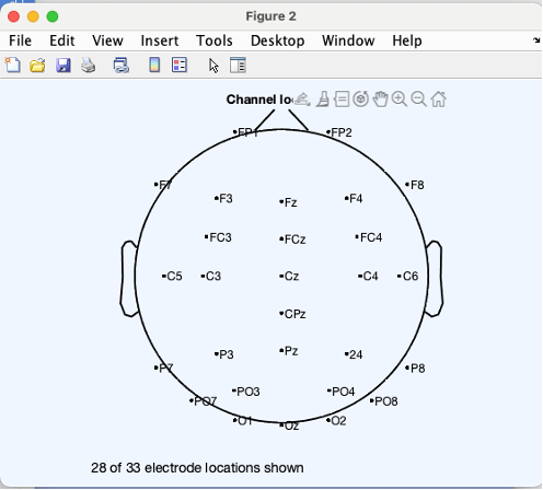
Plot channel locations
- In the EEGLAB graphic user interface (GUI). Go to file > load existing dataset. Select “1_P3_shifted_ds_reref_ucbip.set”
- In EEGLAB GUI, Go to Plot > Channel locations > By name. You should see a simple scalp map with 28 of the 33 electrode locations plotted. (The locations for the reference electrodes and EOG electrodes are not shown)
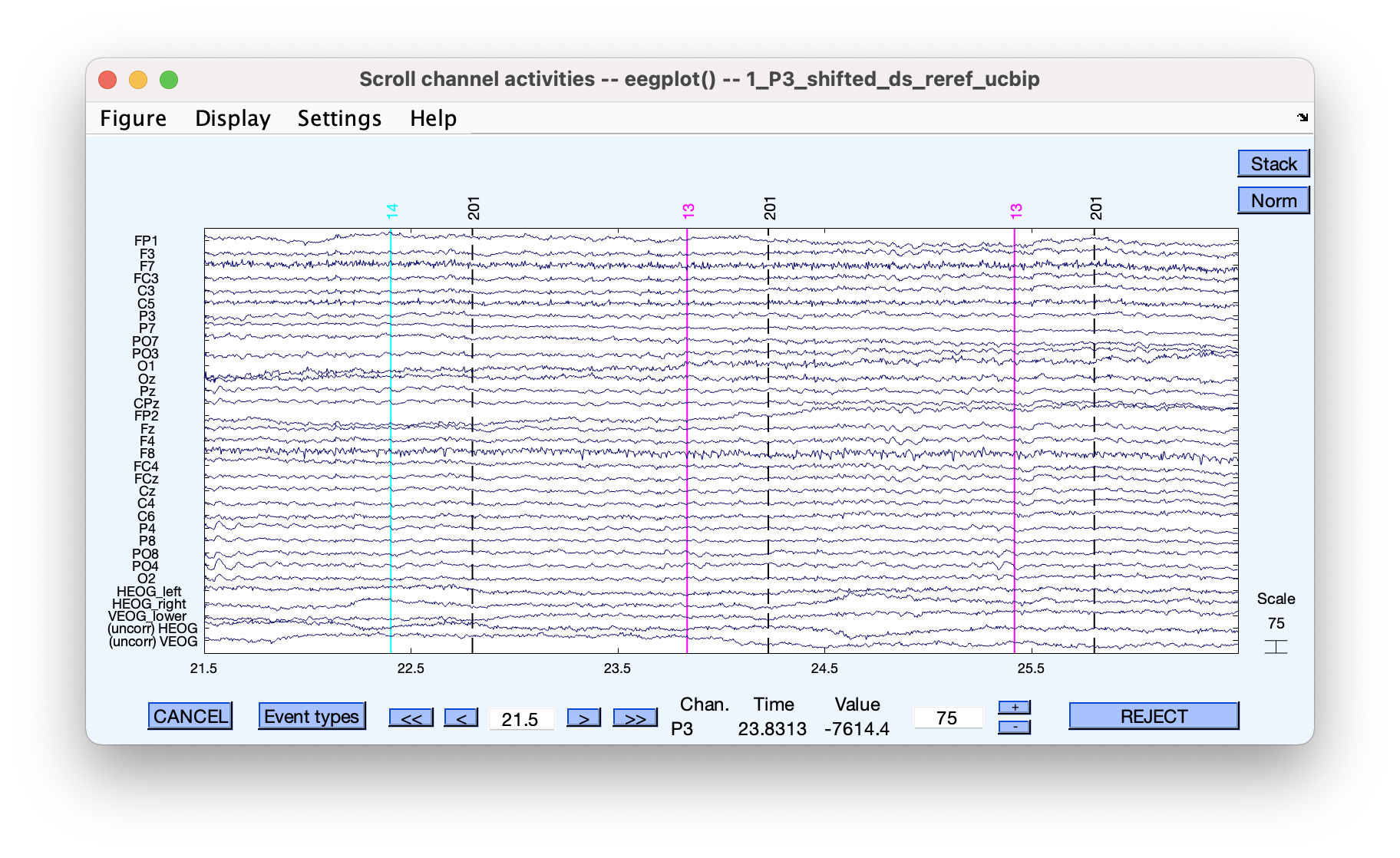
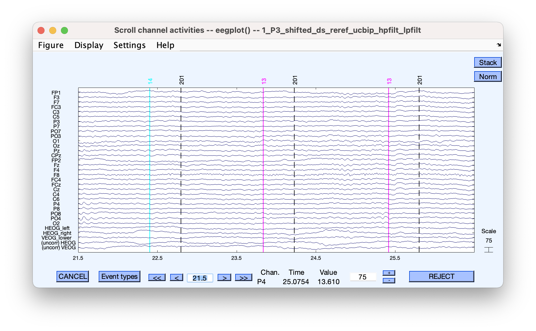
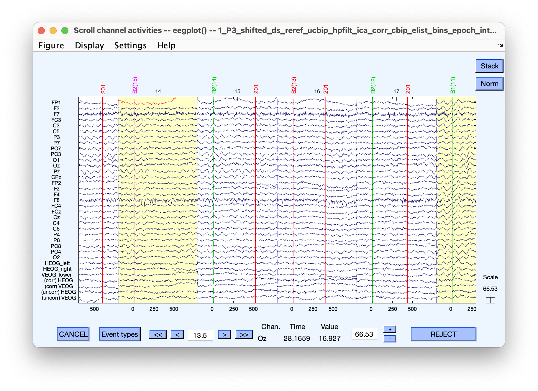
Plot channel data (scroll)
- Go to Plot > Channel data (scroll)
- In pop-up window select Display > remove DC offset
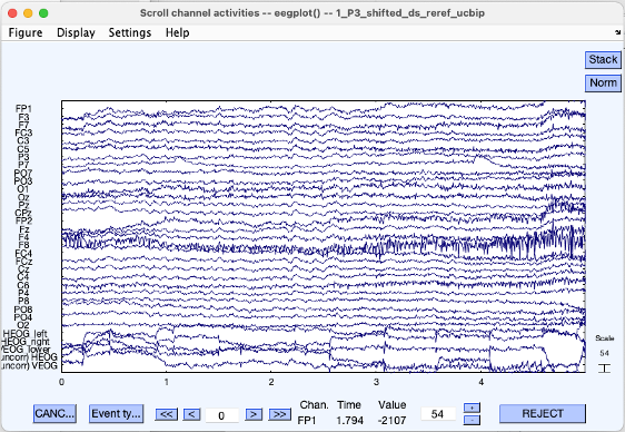
You should see recordings from each channel after the DC offset has been removed. (DC offset EEG recording systems refers to general low-frequency drift in the recordings due to the electrode-tissue interface.) Try finding some of the common artifacts like blinks/eye-movements, alpha waves, muscle noise
This is also a good time to remove bad channels (e.g. broken electrodes, high impedance electrodes) from your data based on visual examination.
1
2
3
4
%Interpolate bad channels
%create or load in list of bad channels from a .txt
bad_chans = [1 11 21]
EEG = pop_interp(EEG, [bad_chans], 'spherical');
Step 2: Filter
High-pass filters are best applied to continuous EEG data to avoid distorting the edges at the beginning and end of epochs.
1
2
3
%Remove DC offsets and apply a high-pass filter (non-causal Butterworth impulse response function, 0.1 Hz half-amplitude cut-off, 12 dB/oct roll-off)
EEG  = pop_basicfilter( EEG,  1:33 , 'Boundary', 'boundary', 'Cutoff',  0.1, 'Design', 'butter', 'Filter', 'highpass', 'Order',  2, 'RemoveDC', 'on' );
[ALLEEG EEG CURREN TSET] = pop_newset(ALLEEG, EEG, 2, 'setname', ['1_P3_ds_reref_ucbip_hpfilt']);
Check your data
How did your filter affect it?
Pre-Filter
After 0.1 Hz high-pass filter
.) for compelling examples).](/assets/images/2023-04-07-eeg-analysis/data_3.png)
There is not much difference after applying a conservative 0.1 Hz high-pass filter. This is not necessarily a bad thing because aggressive filters can distort the shape and temporal structure of EEG data, sometimes creating large ERP differences that aren’t really there (see this blog post for compelling examples).
Applying 30 Hz low-pass filter for fun
1
2
3
%low-pass filter
EEG  = pop_basicfilter( EEG,  1:33 , 'Boundary', 'boundary', 'Cutoff',  30, 'Design', 'butter', 'Filter', 'lowpass', 'Order',  2);
[ALLEEG EEG CURREN TSET] = pop_newset(ALLEEG, EEG, 3, 'setname', ['1_P3_ds_reref_ucbip_hpfilt_lpflit']);
Low pass filters can be less problematic. A 30 Hz low-pass can sometimes be acceptable if you are not interested in any frequency effects remotely close to 30 Hz.
Step 3: ICA
ICA is an optional, but commonly used, step for identifying and removing well-characterized artifacts, such as blinks, eye movements, and heartbeats. It’s useful because, in theory, you can clean your data without having to delete chunks of it.
You can think of ICA as magic (i.e., math) which separates out a set of activity patterns, in this case defined by scalp distributions, that are maximally statistically independent or stable across time. These activity patterns (components) sum up to account for the EEG recording at any specific time point.
1
2
%Compute ICA weights with runICA
EEG = pop_runica(EEG,'extended',1,'chanind', [1:31]);
This takes forever to run, so we will look at a dataset with ICA weights already calculated.
Examine ICA Components
- File > load existing dataset. Select “1_P3_shifted_ds_reref_ucbip_hpfilt_ica_prep2_weighted.set” from subject folder.
- Note: as an optional step, this dataset has been prepped for ICA using code that removes the breaks in between blocks by identifying and removing 1) long time windows without event codes and 2) time windows with huge movement artifacts
- Because we’ve jumped around in the processing stream, we need to load channel locations again before we plot the ICA components. Let’s do this in the GUI this time. Go to Edit > Channel locations. Click on the “…” button to open file explorer/finder, navigate to week4_demo and select “standard-10-5-cap385.elp” and click Ok. Click Ok again in the pop-up window titled Edit channel info to accept all defaults.
- Plot ICA components with Tools > Inspect/Label components by map. What are some ICA components that look like alpha activity? What looks like a blink?
- Mark a blink component for rejection. Go to Tools > Remove components from data. When given the option, click “Plot single trials” to look at channel scroll data with (blue) and without (red) that ICA component.
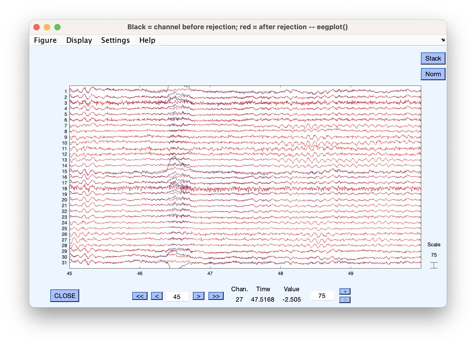
Component 2 was marked for rejection in this example
You can see here that the data has been nicely “reconstructed” without a specific activity pattern (blinks) that we did not want. In theory this means we can get clean data without having to discard every segment with artifacts.
Code for doing this programmatically after loading in a csv file with components to reject for each subject:
1
2
3
4
5
6
7
8
9
10
11
12
13
14
15
16
17
18
%Load list of ICA component(s) corresponding to ocular artifacts from Excel file ICA_Components_P3.xlsx
[ndata, text, alldata] = xlsread([Current_File_Path filesep 'ICA_Components_P3']);
MaxNumComponents = size(alldata, 2);
    for j = 1:length(alldata)
        if isequal(SUB{i}, num2str(alldata{j,1}));
            NumComponents = 0;
            for k = 2:MaxNumComponents
                if ~isnan(alldata{j,k});
                    NumComponents = NumComponents+1;
                end
                Components = [alldata{j,(2:(NumComponents+1))}];
            end
        end
    end

%Perform ocular correction by removing the ICA component(s) specified above
EEG = pop_subcomp( EEG, [Components], 0);
[ALLEEG EEG CURRENTSET] = pop_newset(ALLEEG, EEG, 2,'setname',[SUB{i} '_P3_shifted_ds_reref_ucbip_hpfilt_ica_corr'],'savenew', [Subject_Path SUB{i} '_P3_shifted_ds_reref_ucbip_hpfilt_ica_corr.set'],'gui','off');
The .csv file looks like this:
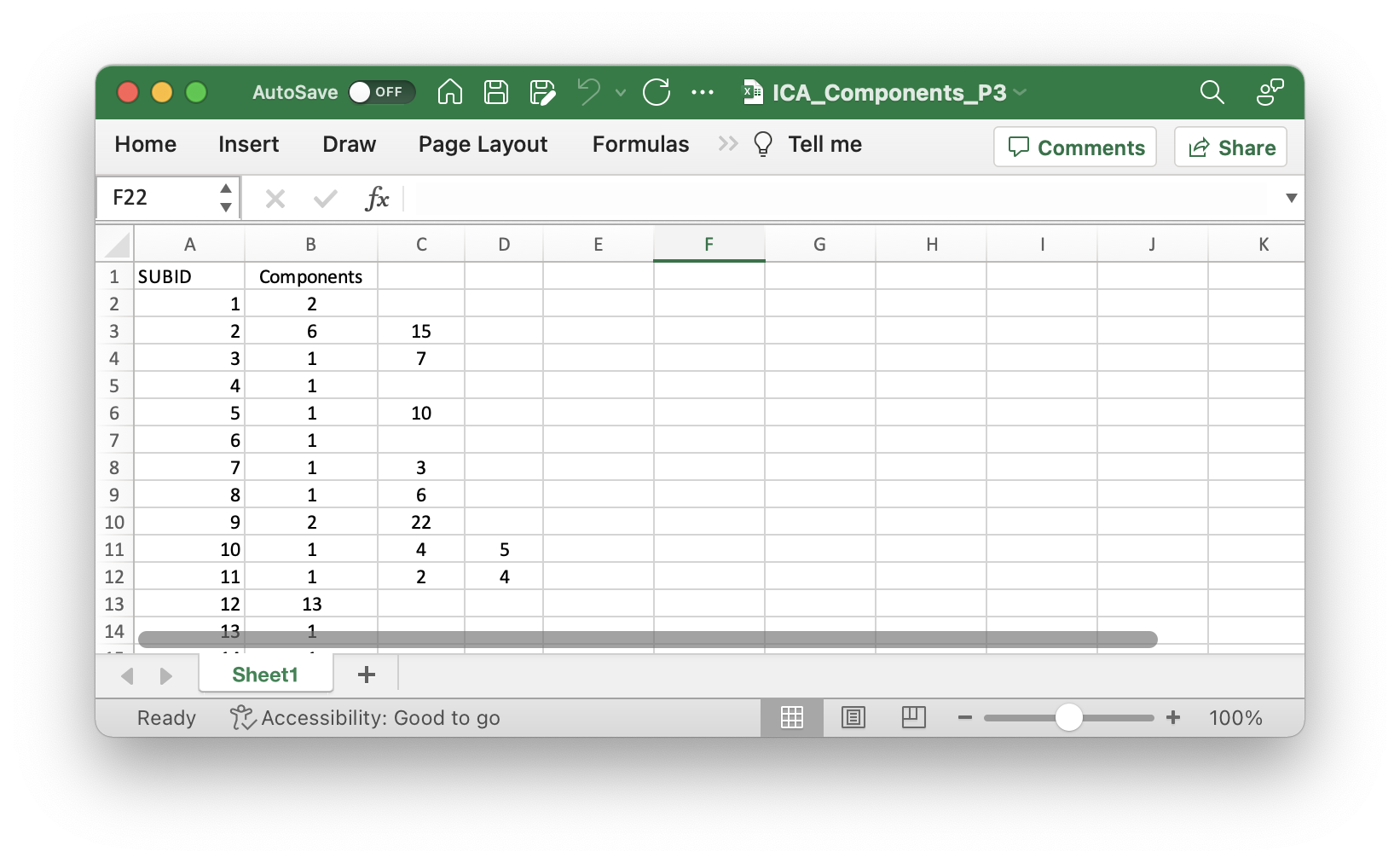
Note: every time you re-run ICA, these components are going to be slightly different because ICA starts with a random weight matrix. After you’ve manually identified your components, avoid running ICA again - it’ll erase all your work!
Step 4: Epoch and Bin
1
2
3
4
5
6
7
8
9
%paths & subj number (set to 1)
Current_File_Path = '/Users/audreyliu/Library/CloudStorage/Box-Box/methods_jc_eeg/P3/EEG_ERP_Processing';
Subject_Path = '/Users/audreyliu/Library/CloudStorage/Box-Box/methods_jc_eeg/P3/data/1/';
SUB = {'1', '2', '3'};
i = 1;

%Create EEG Event List containing a record of all event codes and their timing
EEG  = pop_creabasiceventlist( EEG , 'AlphanumericCleaning', 'on', 'BoundaryNumeric', { -99 }, 'BoundaryString', { 'boundary' }, 'Eventlist', [Subject_Path SUB{i} '_P3_Eventlist.txt'] );
[ALLEEG EEG CURRENTSET] = pop_newset(ALLEEG, EEG, 2, 'setname', [SUB{i} '_P3_shifted_ds_reref_ucbip_hpfilt_ica_corr_cbip_elist'], 'savenew', [Subject_Path SUB{i} '_P3_shifted_ds_reref_ucbip_hpfilt_ica_corr_cbip_elist.set'], 'gui', 'off');
This outputs an “event list” which is a .txt file like this:
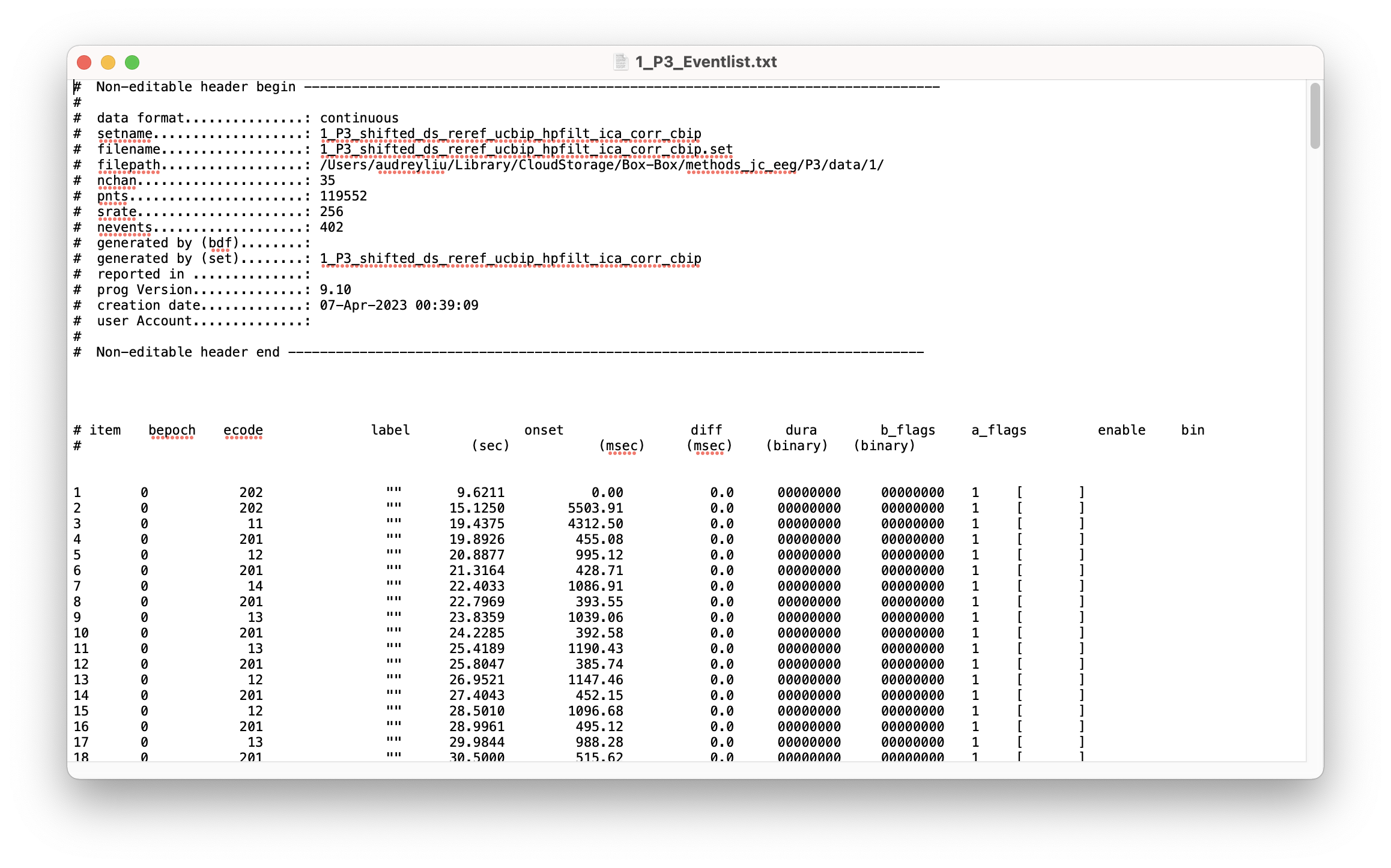
The “bin” column is empty because we haven’t told MATLAB which event codes represent which conditions yet. Let’s load in the bin description file (BDF_P3.txt) which contains this information.
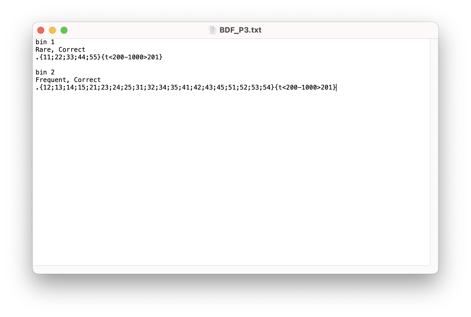
1
2
3
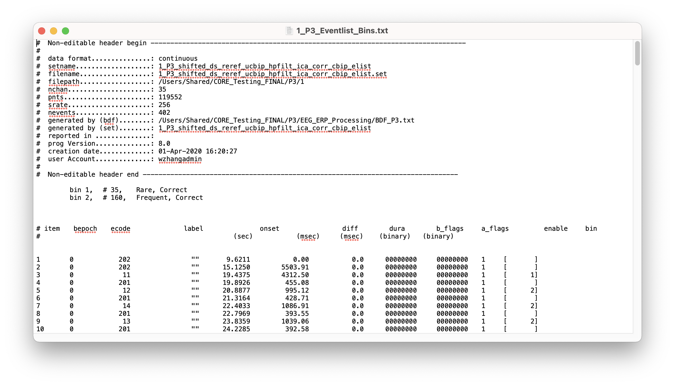
%Assign events to bins with Binlister; an individual trial may be assigned to more than one bin (bin assignments can be reviewed in each subject's P3_Eventlist_Bins.txt file)
EEG = pop_binlister( EEG , 'BDF', [Current_File_Path filesep 'BDF_P3.txt'], 'ExportEL', [Subject_Path SUB{i} '_P3_Eventlist_Bins.txt'], 'IndexEL', 1, 'SendEL2', 'EEG&Text', 'UpdateEEG', 'on', 'Voutput', 'EEG' );
[ALLEEG EEG CURRENTSET] = pop_newset(ALLEEG, EEG, 3, 'setname', [SUB{i} '_P3_shifted_ds_reref_ucbip_hpfilt_ica_corr_cbip_elist_bins'], 'savenew', [Subject_Path SUB{i} '_P3_shifted_ds_reref_ucbip_hpfilt_ica_corr_cbip_elist_bins.set'], 'gui', 'off');
Now our bins are labelled and we also have a new event list file for this subject ‘1_P3_Eventlist_Bins.txt’ with bins filled in:
Next, let’s cut our data into trial epochs
1
2
3
%Epoch the EEG into 1-second segments time-locked to the response (from -200 ms to 800 ms) and perform baseline correction using the average activity from -200 ms to 0 ms
EEG = pop_epochbin( EEG , [-200.0  800.0],  [-200.0  0.0]);
[ALLEEG EEG CURRENTSET] = pop_newset(ALLEEG, EEG, 4, 'setname', [SUB{i} '_P3_shifted_ds_reref_ucbip_hpfilt_ica_corr_cbip_elist_bins_epoch'], 'savenew', [Subject_Path SUB{i} '_P3_shifted_ds_reref_ucbip_hpfilt_ica_corr_cbip_elist_bins_epoch.set'], 'gui', 'off');
Step 6: Artifact Detection
Artifact detection and rejection is another data cleaning step where we delete whole epochs that contain large artifacts.
There are, again, many different methods for artifact detection (this is a theme). For this example, we will use the moving window peak-to-peak amplitude function.
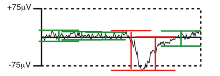
How moving window peak-to-peak amplitude detection works. Since we’re measuring amplitudes with a moving window, slow, low frequency drifts in large segments of data does not get flagged as artifacts.
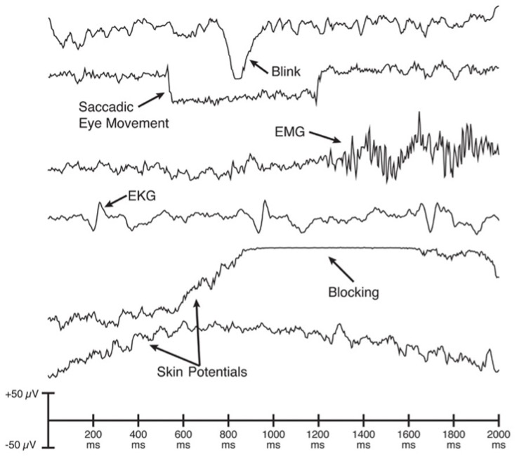
Commonly Recorded Artifactual Potentials (C.R.A.P)
Unique window sizes and thresholds are used for each subject to account for individual variability in the size of their signals
1
2
3
4
5
6
7
8
9
10
11
12
13
14
15
16
17
18
19
20
21
22
%Load the Excel file with the list of thresholds and parameters for identifying C.R.A.P. with the moving window peak-to-peak algorithm for each subject
[ndata3, text3, alldata3] = xlsread([Current_File_Path filesep 'AR_Parameters_for_MW_CRAP_P3']);

%Identify segments of EEG with C.R.A.P. artifacts using the moving window peak-to-peak algorithm with the parameters in the Excel file for this subject
    DimensionsOfFile3 = size(alldata3);
    for j = 1:DimensionsOfFile3(1)
        if isequal(SUB{i},num2str(alldata3{j,1}));
            if isequal(alldata3{j,2}, 'default')
                Channels = 1:28;
            else
                Channels = str2num(alldata3{j,2});
            end
            Threshold = alldata3{j,3};
            TimeWindowMinimum = alldata3{j,4};
            TimeWindowMaximum = alldata3{j,5};
            WindowSize = alldata3{j,6};
            WindowStep = alldata3{j,7};
        end
    end

    EEG  = pop_artmwppth( EEG , 'Channel',  Channels, 'Flag', [1 3], 'Threshold', Threshold, 'Twindow', [TimeWindowMinimum  TimeWindowMaximum], 'Windowsize', WindowSize, 'Windowstep', WindowStep );
    [ALLEEG EEG CURRENTSET] = pop_newset(ALLEEG, EEG, 4, 'setname', [SUB{i} '_P3_shifted_ds_reref_ucbip_hpfilt_ica_corr_cbip_elist_bins_epoch_interp_SVT_MW1'], 'gui', 'off');
Plot new dataset to see if the tagged epochs look like they were tagged for a good reason.
This one looks like it might be a blink.
Step 7: Computing individual subject ERPs
1
2
3
%Create an averaged ERP waveform
ERP = pop_averager( EEG , 'Criterion', 'good', 'ExcludeBoundary', 'on', 'SEM', 'on');
ERP = pop_savemyerp( ERP, 'erpname', [SUB{i} '_P3_erp_ar_test'], 'filename', [Subject_Path SUB{i} '_P3_erp_ar_test.erp']);
Optional but suggested step: check percentage of trials rejected in total and per bin.
1
2
3
4
5
6
7
8
9
10
11
12
13
14
15
16
17
18
19
%Calculate the percentage of trials that were rejected in each bin
accepted = ERP.ntrials.accepted;
rejected= ERP.ntrials.rejected;
percent_rejected= rejected./(accepted + rejected)*100;

%Calculate the total percentage of trials rejected across all trial types (first two bins)
total_accepted = accepted(1) + accepted(2);
total_rejected= rejected(1)+ rejected(2);
total_percent_rejected= total_rejected./(total_accepted + total_rejected)*100;

%Save the percentage of trials rejected (in total and per bin) to a .csv file
fid = fopen([Subject_Path filesep SUB{i} '_AR_Percentages_P3_test.csv'], 'w');
fprintf(fid, 'SubID,Bin,Accepted,Rejected,Total Percent Rejected\n');
fprintf(fid, '%s,%s,%d,%d,%.2f\n', SUB{i}, 'Total', total_accepted, total_rejected, total_percent_rejected);
bins = strrep(ERP.bindescr,', ',' - ');
for b = 1:length(bins)
    fprintf(fid, ',%s,%d,%d,%.2f\n', bins{b}, accepted(b), rejected(b), percent_rejected(b));
end
fclose(fid);
Plotting individual subject ERPs
Note: baseline correction is applied here for plotting
1
2
3
4
5
6
7
8
9
10
11
12
13
14
15
16
17
18
19
20
21
22
%Set baseline correction period in milliseconds
baselinecorr = '-200 0';

%Set x-axis scale in milliseconds
xscale = [-200.0 800.0   -200:200:800];

%Set y-axis scale in microvolts for the EEG channels for the parent waves
yscale_EEG_parent = [-20.0 50.0   -20:10:50];

%Set y-axis scale in microvolts for the EEG channels for the difference waves
yscale_EEG_diff = [-20.0 30.0   -20:10:30];

%Load the low-pass filtered averaged ERP waveforms outputted from Script #7 in .erp ERPLAB file format
ERP = pop_loaderp('filename', [SUB{i} '_P3_erp_ar_diff_waves_lpfilt.erp'], 'filepath', Subject_Path);

%Plot the P3 rare and frequent parent waveforms at the key electrode sites of interest (FCz, Cz, CPz, Pz)
ERP = pop_ploterps( ERP, [1 2], [20 21 14 13] , 'Box', [2 2], 'blc', baselinecorr, 'Maximize', 'on', 'Style', 'Classic', 'xscale', xscale,  'yscale', yscale_EEG_parent);
save2pdf([Subject_Path 'graphs' filesep SUB{i} '_P3_Parent_Waves.pdf']);

%Plot the P3 rare-minus-frequent difference waveform at the key electrode sites of interest (FCz, Cz, CPz, Pz)
ERP = pop_ploterps( ERP, [3], [20 21 14 13] , 'Box', [2 2], 'blc', baselinecorr, 'Maximize', 'on', 'Style', 'Classic', 'xscale', xscale,  'yscale', yscale_EEG_diff);
save2pdf([Subject_Path 'graphs' filesep SUB{i} '_P3_Difference_Wave.pdf']);
Step 8: Grand Averaging
See ERP-CORE script for reference:
Outro
There are many ways to preprocess EEG data - EEGLAB/ERPLAB is a nice starting point for beginners and workshops/classes because it is easy to visualize steps and skip back and forth in the processing stream.
Fieldtrip is another MATLAB package (see Mike X Cohen book below). It uses slightly more complicated data structures, but I think it is much more effective for statistics and plotting (and certainly for time-frequency analyses).
No matter what you go with, it is important to decide on an analysis pipeline before looking at (or even collecting) your data to avoid ‘creating’ effects through tweaking analysis parameters.
References
Full ERP-CORE Tutorial (download working analysis scripts here)
EEGLAB Wiki - Step 5. Preprocess data
Other resources
Installing MATLAB/EEGLAB/ERPLAB for dummies:
Guide for using fieldtrip for EEG preprocessing and more:
Mike X Cohen - Analyzing Neural Time Series Data
One new methods paper comparing different EEG preprocessing pipelines: