A too-brief overview of this powerful and (usually) intuitive approach
to statistical computing.
Downloading & using R
One of the biggest virtues of R is that it’s completely open-source and
free to use. This is really important if we care about making our work
reproducible and/or making science more accessible – people can’t
(easily) make use of your work if they have to pay hundreds of dollars
in licensing fees or be affiliated with a university that covers them!
New versions of R are constantly being released. In 2020 alone, they’ve
put out 5 different versions (one big switch from 3.6.3 –> 4.0.0 and
the rest tweaks on 4.0). You don’t need to always have the most
up-to-date version, but if you’re downloading R for the first time today
you might as well get 4.0.2. In
general, it’s good practice to not let your R version get too far behind
what’s being released, but I don’t recommend doing this while you’re in
the middle of a project or on a tight deadline. Switching versions can
lead to previously written code not working properly, and you have to
reinstall all your packages after you update (though see this brief
script that
nicely streamlines the process).
To IDE or not to IDE?
…is a question of personal preference. Most people choose to use the
RStudio IDE, which you can download here. Others
use a text editor (e.g., Atom) to write scripts that
you can run via Terminal. I personally love RStudio and am more than
happy to field any questions / share my hacks with anyone who is
interested.
Once you have the R software on your computer and some way to open &
edit .R files, then you are ready to start using R!
Data types & structures
There are 6 main datatypes that you’ll encounter while using R:
- character:
'hello world'
- numeric:
2020, 40.5
- integer:
1L, 2L (L tells R to store the value as an integer;
the L doesn’t show up when you print out the actual values)
- logical:
TRUE, FALSE
- complex:
1+6i (numbers with real & imaginary parts)
You can coerce a variable from one type to another by using the
as.<type> command:
1
2
| y <- as.character(x)
y
|
There are 5 main data structures that you’ll encounter while using
R:
- atomic vector: a set of elements of the same type
- matrix: an atomic vector with dimensions of row, column
- list: a set of elements that can be different types (even other
lists)
- data frame: a “rectangular” list where every element has the
same length
- factors: a dataframe element whose integer values have a
corresponding set of character values that display instead of the
integer; used in the case of categorical variables
Atomic vectors
There are lots of ways to create atomic vectors. What you’ll most
commonly see used is the c() (for combine) function:
1
2
3
| numeric_vector <- c(1,2,3,4)
character_vector <- c('intro', 'to', 'R', 'and', 'Tidyverse')
numeric_vector
|
1
| ## [1] "intro" "to" "R" "and" "Tidyverse"
|
rep() and seq() are really handy ways to create vectors as well:
1
2
| repeat_a_range <- rep(1:10, 5)
repeat_a_range
|
1
2
| ## [1] 1 2 3 4 5 6 7 8 9 10 1 2 3 4 5 6 7 8 9 10 1 2 3 4 5
## [26] 6 7 8 9 10 1 2 3 4 5 6 7 8 9 10 1 2 3 4 5 6 7 8 9 10
|
1
| create_a_sequence <- seq(1, 10, 0.5)
|
You can use the c() function to add onto existing vectors:
1
2
| new_vector <- c(100, numeric_vector, 25)
new_vector
|
You index vectors with brackets and the position of the element you want
to extract. One big difference between R and Python is indexing: R does
not use zero-indexing and is inclusive on the second. So to access the
first element of a structure, you use 1 and to access the nth, you use
n.
1
2
| # what's the best programming language?
character_vector[3]
|
Matrices
I’ve personally never worked directly with a matrix in R – it’s either
dataframes or lists. When doing PCA, for example, I just use a package
that does the SVD for me and outputs the results into a list. But they
follow the same rules for indexing as any other language:
1
2
3
| # matrices are filled column-wise
m <- matrix(1:6, nrow = 3, ncol = 2)
m
|
1
2
3
4
| ## [,1] [,2]
## [1,] 1 4
## [2,] 2 5
## [3,] 3 6
|
1
2
3
| # you can transform vectors to matrices pretty easily
dim(new_vector) <- c(2,3)
new_vector
|
1
2
3
| ## [,1] [,2] [,3]
## [1,] 100 2 4
## [2,] 1 3 25
|
1
2
| # index them using [row, column]
new_vector[2,3]
|
1
2
3
| # and you can combine vectors into matrices using cbind() or rbind()
new_matrix <- cbind(repeat_a_range, numeric_vector)
length(new_matrix[1,])
|
Lists
The most liberal of all R data types, lists are basically just a bucket
to dump stuff into. There’s no requirement that the data types match (as
in atomic vectors) or that elements be of the same size (as in
dataframes). For this reason, a good amount of packages that run
advanced stats (e.g., lme4, prcomp) will dump their results into a list.
1
2
3
| list <- list(4, 'b', FALSE)
# all that flexibility comes at the cost of indexing efficiency -- you need double brackets to extract a specific element
list[[3]]
|
1
2
3
| # elements of a list can have be named
named_list <- list(numbers = 1:4, letters = c('a','b','c','d'), booleans = rep(c(T,F),2))
named_list
|
1
2
3
4
5
6
7
8
| ## $numbers
## [1] 1 2 3 4
##
## $letters
## [1] "a" "b" "c" "d"
##
## $booleans
## [1] TRUE FALSE TRUE FALSE
|
1
2
| # but then you index them with $ instead of brackets. still use brackets to index elements inside of a sublist though
named_list$letters[2]
|
Dataframes
The crown jewel of R. It’s the primary way you’ll interact with tabular
data. Making a dataframe from scratch is super easy:
1
2
3
| df <- data.frame(subID = 1:10, x = seq(10, 100, 10), y = 25:34)
# preview the first 6 rows by calling
head(df)
|
1
2
3
4
5
6
7
| ## subID x y
## 1 1 10 25
## 2 2 20 26
## 3 3 30 27
## 4 4 40 28
## 5 5 50 29
## 6 6 60 30
|
Now for the real fun: working with actual data. In order to store your
data for future use, you need to save it as a variable. Reading in
tabular data with read.csv() will automatically assign it as a data
frame. It also defaults to interpreting strings as factors, which can be
annoying (especially if you’re working with a Qualtrics file, because
the first row is a character so all of your variables become factors),
so it’s good practice to add stringsAsFactors = F to the read.csv()
call. And formally noting here that variable values are assigned using
<- in R.
1
2
3
| df <- read.csv('2020-10-14-data.csv', stringsAsFactors = F)
# get a statistical overview of your data by calling
summary(df)
|
1
2
3
4
5
6
7
| ## ID steps bmi sex
## Min. : 1.0 Min. : 0 Min. :15.00 Length:1786
## 1st Qu.: 447.2 1st Qu.: 5301 1st Qu.:20.93 Class :character
## Median : 893.5 Median : 7431 Median :26.80 Mode :character
## Mean : 893.5 Mean : 7435 Mean :25.29
## 3rd Qu.:1339.8 3rd Qu.: 9699 3rd Qu.:29.30
## Max. :1786.0 Max. :15000 Max. :32.00
|
1
2
| # get a structural overview by calling
str(df)
|
1
2
3
4
5
| ## 'data.frame': 1786 obs. of 4 variables:
## $ ID : int 1 2 6 7 8 10 11 13 17 18 ...
## $ steps: int 15000 15000 14861 14861 14699 14560 14560 14560 14560 14560 ...
## $ bmi : num 16.9 16.9 16.8 16.8 17.3 20.5 20.6 20.5 20.4 20.4 ...
## $ sex : chr "M" "M" "M" "M" ...
|
1
2
| # access a column with $; tail() returns the last 6 values (or rows, if you call it on a df)
tail(df$ID)
|
1
| ## [1] 1781 1782 1783 1784 1785 1786
|
Factors
When you think about how data is typically set up, it makes sense for
stringsAsFactors = T to be the default in read.csv(). Usually, we
use character values to define levels of a categorical variable. And
that’s precisely the data type of a factor: an integer (think dummy
coding) that has a corresponding character label.
One of my favorite tricks for checking if some data mutation or
filtering procedure worked is to call
1
| levels(as.factor(df$sex))
|
I find this really convenient for quickly checking out all of the values
of a given variable. And since we don’t save this call by assigning it
to a column in the df, it’s completely transient (and thus useful for
all different kinds of data types). But it seems like sex is the kind of
thing that we’d want to use as a catgeorical variable. Here’s how you do
that:
1
2
3
| df$sex <- factor(df$sex, levels = c('M', 'F'), labels = c('Male', 'Female'))
# the levels argument allows you to modify the order of the levels, and the labels argument allows you to change what string is presented when you index a particular level
levels(df$sex)
|
Shoutout to software carpentry, whose
webpage on data type &
structures
helped me a bunch when putting this portion of the workshop together.
Now that we’re familiar with the most common data structures & types, we can start exploring the
What the heck is a Tidyverse?
“The tidyverse is an opinionated collection of R packages designed for
data science. All packages share an underlying design philosophy,
grammar, and data structures.” ~
tidyverse.org
The abundance of packages available to an R programmer is arguably the
best thing about the language. The packages in the tidyverse are so
popular that understanding their syntax is pretty much necessary if you
want to be able to use other people’s code. We don’t have time to get
into every single package today, so we’ll focus on dplyr and
ggplot2.
A quick note about packages. None come pre-installed with the base R
software or an IDE, so all must first be added to a library by running
install.packages("packagename"). This only needs to be done once, but
every time you start a new session, you need to load in the packages
that you plan to use. So if you don’t already have the tidyverse
installed on your machine, you first need to run
install.packages('tidyverse'). Then,
If you’re only using one or two packages from the ’verse, then you
probably don’t need to load in the whole thing. You can just call
library(ggplot2) for instance. But I typically use functions from 4+
different libraries, so I find it more succinct to call in the whole
thing.
While getting accustomed to the different functions available to me (and
even when trying to do something I haven’t done before), these
cheatsheets were an absolute
godsend. I have copies of the data
transformation
and data
visualization
sheets on every computer I use. Sometimes Google/StackOverflow will be
better for a very specific question, but I think these are unparalleled
for getting a birds-eye view of all the functionality at your
fingertips.
Tidy data
Central to the tidyverse is the concept of a “tidy”
dataframe. This is
a df that’s structured in such a way that every column is a variable and
every row is an observation. All the following examples assume that data
is organized like this (because it uses a df that is indeed tidy).
If dataframes are the crown jewel of R, then my personal opinion is that
dplyr is the queen upon whose head the crown rests (sorry lol). It
gives you a collection of functions that are incredibly useful for
working with and manipulating dataframes. It’s also responsible for what
I think is one of the most powerful operators, the pipe %>%.
filter()
Piping is one of the big syntactical advances introduced by tidyverse.
Instead of constantly having to call up the variable that stores your
df, it allows you to call it once and then ‘pipe’ it through the rest of
your transformations. Here’s an example using the filter() function,
which allows you to select cases that meet different logical conditions:
1
| df %>% filter(sex == 'Female' & ID %in% c(1:5))
|
1
2
3
4
| ## ID steps bmi sex
## 1 3 15000 17.0 Female
## 2 4 14861 17.2 Female
## 3 5 14861 17.2 Female
|
So here we have a subset of our dataframe that contains only the
observations from females whose subject IDs are in the range 1:5. Notice
that we didn’t have to preface our index of a column with df$. This is
because we’ve piped the df into the filter() function. We could
achieve the same thing by calling filter(df, sex == 'Female' & ID %in%
c(1:5)). In either case, you don’t need to enclose your variable names
with '' in the tidyverse.
Let’s see what happens when we call
1
2
3
4
5
6
7
| ## ID steps bmi sex
## 1 1 15000 16.9 Male
## 2 2 15000 16.9 Male
## 3 6 14861 16.8 Male
## 4 7 14861 16.8 Male
## 5 8 14699 17.3 Male
## 6 10 14560 20.5 Male
|
We lost our transformation because we didn’t save it as a variable. Just
like the levels(as.factor(var$df)) call, piping on its own results in
a transient (i.e., one-time) transformation of the data that isn’t
stored anywhere. Usually, I like to keep one copy of the raw data in my
workspace so that I don’t need to read in the csv every time I want to
backtrack my steps. So if we want to create a new df that only contains
observations from females, we need to save it as its own variable:
1
2
| df_female <- df %>% filter(sex == 'Female')
summary(df_female)
|
1
2
3
4
5
6
7
| ## ID steps bmi sex
## Min. : 3.0 Min. : 0 Min. :15.00 Male : 0
## 1st Qu.: 538.0 1st Qu.: 4699 1st Qu.:21.60 Female:921
## Median : 990.0 Median : 7130 Median :27.30
## Mean : 968.5 Mean : 6891 Mean :25.66
## 3rd Qu.:1419.0 3rd Qu.: 9259 3rd Qu.:29.50
## Max. :1786.0 Max. :15000 Max. :32.00
|
select()
If I want to create a new df that’s a subset of variables (columns),
then I can use select():
1
2
| # let's say I want a look at the data without knowing anything about sex
df %>% select(ID, steps, bmi) %>% head()
|
1
2
3
4
5
6
7
| ## ID steps bmi
## 1 1 15000 16.9
## 2 2 15000 16.9
## 3 6 14861 16.8
## 4 7 14861 16.8
## 5 8 14699 17.3
## 6 10 14560 20.5
|
1
| # see how I can pipe this interim dataset into a base R function? super neat!
|
A great thing about the pipe is that it works with all kinds of
functions, not just dplyr or tidyerse ones. And you can pipe
anything – I often pipe the outputs of emmeans() (a list) into
as.data.frame() when I want to make a quick plot of mixed model
estimates (more on this next meeting).
select() also has a whole host of helper functions that are great for
working with dfs that have a bunch of columns. Some examples are
indexing by variable prefix (starts_with()) or suffix (ends_with()),
and string matching (contains() for a literal string, matches() for
a regular expression).
You can also tell select() to pick out all of the variables except
those in a particular vector by using -c(var1, var2, etc.). And of
course, you can combine all of these syntaxes into one long select()
call to keep things neat.
group_by(), mutate(), and summarise()
Suppose that in addition to creating subsets of my df, I also want to
compute some values based on those subsets, or even make a separate df
with relevant summary stats. In this case, group_by(), mutate(), and
summarise() are your friends.
group_by() allows you to stratify your dataset by any desired grouping
variable and then perform transformations on this new group basis.
mutate() (or its more chaotic cousin, transmute()) are what allow
you to make those transformations. mutate() creates a new variable
that’s a function of existing variables, whereas transmute() replaces
the existing variables with the new one.
1
2
3
4
| df %>%
group_by(ID) %>%
mutate(mean_bmi = mean(bmi)) %>%
head()
|
1
2
3
4
5
6
7
8
9
10
| ## # A tibble: 6 x 5
## # Groups: ID [6]
## ID steps bmi sex mean_bmi
## <int> <int> <dbl> <fct> <dbl>
## 1 1 15000 16.9 Male 16.9
## 2 2 15000 16.9 Male 16.9
## 3 6 14861 16.8 Male 16.8
## 4 7 14861 16.8 Male 16.8
## 5 8 14699 17.3 Male 17.3
## 6 10 14560 20.5 Male 20.5
|
Since this is a dataset where each individual contributed one
observation, mutate() isn’t that useful. But if you have repeated
observations from participants and want to compute some mean value per
participant (e.g., proportion correct), group_by(subID) %>%
mutate(propCorrect = mean(accuracy)) is the way to go. And if you get
some errors because of missing values, just pop in na.rm=T to the
mean() call and you’ll be all good.
While grouping is great for some things, it can cause some weird issues
down the line / under the hood. So it’s typically advised to ungroup()
your df once you’re done transforming it.
summarise() is perhaps the most “chaotic” of all of these functions
because, whereas transmute() replaces the variables that you’re
computing over with the new one you’re creating, summarise() creates a
completely new dataset that includes only the variables that you specify
in the call. This is why I always save any transformation including
summarise() as a new variable – don’t want to overwrite the main df
you’re tidying that has rows for every observation.
1
2
3
4
5
| sex_means <- df %>%
group_by(sex) %>%
summarise(mean_steps = mean(steps),
mean_bmi = mean(bmi))
sex_means
|
1
2
3
4
5
| ## # A tibble: 2 x 3
## sex mean_steps mean_bmi
## <fct> <dbl> <dbl>
## 1 Male 8014. 24.9
## 2 Female 6891. 25.7
|
You’re obviously not limited to just taking means when you use
summarise(). You can perform whatever function you want. For example:
1
2
3
4
| df %>%
summarise(random_value1 = ID*bmi - steps,
random_value2 = steps + bmi^sqrt(ID)) %>%
head()
|
1
2
3
4
5
6
7
| ## random_value1 random_value2
## 1 -14983.1 15016.90
## 2 -14966.2 15054.51
## 3 -14760.2 15864.19
## 4 -14743.4 16606.27
## 5 -14560.6 17873.85
## 6 -14355.0 28624.68
|
That’s all we’ll cover in dplyr today. Again, I can’t emphasize enough
how helpful it is to spend an hour or so studying the data
transformation
cheetsheat
and playing around with some data to get a sense of all the powerful
things dplyr allows you to do.
Data visualization with ggplot2
A package after my own heart. We can (and should) have a whole workshop
dedicated to ggplot2, but today I’ll just be covering the basics.
Something that is frustrating when you’re beginning to work with
ggplot2 is how many lines of code it takes to make a decent-looking
plot. This is a consequence of the fact that ggplot works by
layering different aesthetic mappings of your variables onto a
coordinate space that you define. Here’s the basic anatomy of a ggplot
call:
1
| p <- ggplot(df, aes(x=bmi, y=steps, color=sex, fill=sex))
|
ggplot() initializes the ggplot object. df is the dataframe that’s
supplying values for the mappings. And yes, you can indeed pipe a df
into a ggplot call (df %>% ggplot(aes(x,y, etc)))). The aes()
function sets up the coordinate space (x,y) and can be used to set
global aesthetic mappings.
Different ways of visualizing your values are added on (literally, the
syntax is +) to the ggplot object. You don’t necessarily need to save
your plot as a variable, like I did above, but there are some cases when
it’s useful (e.g., when you’re making a workshop with text interspersed
between code chunks, or merging multiple plots together into a single
figure with patchwork).
To get a sense of how layering works, let’s see what the plot looks like
in its current state:
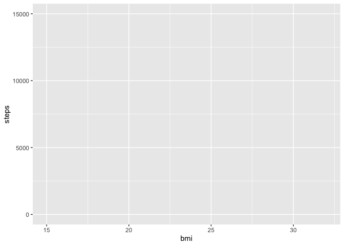
Cool. Now let’s visualize the average amount of steps taken per BMI
class.
1
2
| p +
stat_summary(fun = 'mean', geom='bar', position=position_dodge(1))
|
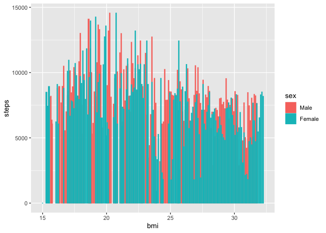
Looks like there’s generally a negative trend between BMI and steps
taken.
stat_summary() is one way to add an aesthetic layer to a ggplot
object. There are a lot of different stat functions that can be really
useful, e.g., if you don’t want to deal with a bunch of different
summarised data frames and would rather compute the stats in your ggplot
calls. Another (and more common) way of adding a layer is to use the
geom family of functions. A geom is just one way of aesthetically
mapping your values onto a plot. In the call above, we used geom='bar'
because we wanted a barplot. We’ll use a geom function in the next
example. Finally, I included position=position_dodge(1) so that the
bars for different sexes weren’t completely on top of each other.
Clearly it didn’t help too much. I should either increase the dodging,
increase the limits of the x axis so the bars have more room to breathe
(xlim(lower, upper)), or use a better geom.
We might get a better sense of the trends in this data by making a
simple scatter plot:
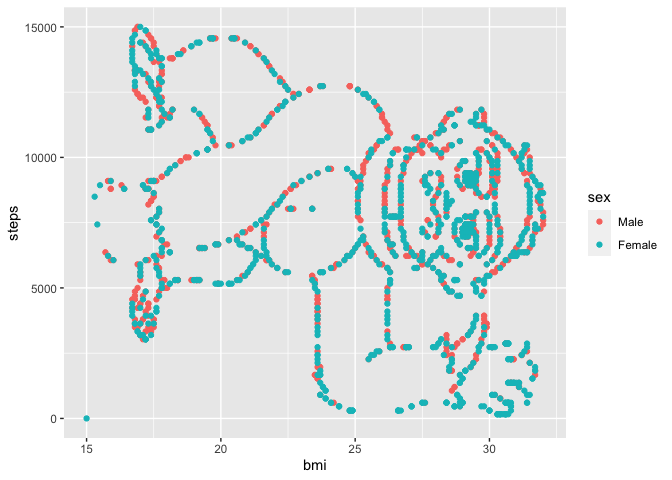
Shoutout to Itai
Yanai on
Twitter for this really fun dataset. A couple things to note: the
gorilla is sideways – we should try flipping our axes so that he’s right
side up. The bars are gone! That’s because we didn’t save that addition
onto the original ggplot object p. Usually you don’t build your plots
in chunks like this, you do everything in one go:
1
2
3
4
5
6
| df %>% ggplot(aes(x=steps, y=bmi, color=sex, fill=sex)) +
geom_point() +
theme_classic() +
scale_color_manual(values = c('mediumpurple1','skyblue')) +
ggtitle('Plot your data!') +
theme(plot.title = element_text(hjust=0.5))
|
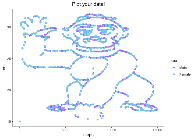
Let’s break down what we did here layer-by-layer.
geom_point() plotted our values as x,y pairstheme_classic() got rid of the gray background and formatted our
axes to look a little more formalscale_color_manual() allowed me to specify the colors that I want
mapped onto the sex variable. I used colors that are built in to
R, but you
can use hex codes or even install packages that have beautiful
palettes.ggtitle() gave our plot a title. we could also use the labs()
argument to set title, x, y, subtitle, etc.- finally,
theme() allowed us to adjust the position of the plot
title. this is one of the beefiest classes of arguments in ggplot,
and also one of the most syntactically verbose. you could spend
hours just reading through ?theme
I cannot emphasize enough just how much more you can do with ggplot.
Like, this barely scratches the surface. For example, you can call
different dataframes to different layers if you want to overlay summary
stats over raw data. You can have differently shaped points for
different levels of a factor, different alpha (transparency) levels as
some value increases, etc. etc.
But for now, I hope that this helped lay the groundwork for the logic of
ggplot and the tidyverse as a whole. Until next time,