
Intro to Mixed Effects Regression in R

Welcome! This is an intro-level workshop about mixed effects regression in R. We’ll cover the basics of linear and logit models. You should have an intermediate-level understanding of R and standard linear regression.
Acknowledgments: Adapted from code provided by Gabriela K Hajduk (gkhajduk.github.io), who in turn referenced a workshop developed by Liam Bailey. Parts of the tutorial are also adapted from a lesson on partial pooling by Tristan Mahr.
For further reading, please check out their tutorials and blogs here:
https://gkhajduk.github.io/2017-03-09-mixed-models/
https://www.tjmahr.com/plotting-partial-pooling-in-mixed-effects-models/
Setup
First, we’ll just get everything set up. We need to tweak some
settings, load packages, and read our data.
1
2
3
4
5
6
7
8
9
10
11
12
13
14
15
16
#change some settings
options(scipen=999) #turn off scientific notation
options(contrasts = c("contr.sum","contr.poly")) #this tweaks the sum-of-squares settings to make sure the output of Anova(model) and summary(model) are consistent and appropriate when a model has interaction terms

#time to load some packages!
library(lme4) #fit the models
library(lmerTest) #gives p-values and more info
library(car) #more settings for regression output
library(dplyr) #for data wrangling
library(tibble) #for data wrangling
library(sjPlot) #plotting model-predicted values
library(ggplot2) #plotting raw data
library(data.table) #for pretty HTML tables of model parameters

#load the data
dragons <- read.csv("2020-10-21-dragon-data.csv")
Data
Let’s get familiar with our dataset. This is a fictional dataset
about dragons. Each dragon has one row. We have information about each
dragon’s body length and cognitive test score. Let’s say our first
research question is whether the length of the dragon is related to its
intelligence.
We also have some other information about each dragon: We know about the mountain range where it lives, color, diet, and whether or not it breathes fire.
Take a look at the data and check the counts of our variables.
1
2
#take a peek at the header
head(dragons)
1
2
3
4
5
6
7
##    testScore bodyLength mountainRange color      diet breathesFire
## 1  0.0000000   175.5122      Bavarian  Blue Carnivore            1
## 2  0.7429138   190.6410      Bavarian  Blue Carnivore            1
## 3  2.5018247   169.7088      Bavarian  Blue Carnivore            1
## 4  3.3804301   188.8472      Bavarian  Blue Carnivore            1
## 5  4.5820954   174.2217      Bavarian  Blue Carnivore            0
## 6 12.4536350   183.0819      Bavarian  Blue Carnivore            1
1
2
3
4
5
#view the full dataset
#View(dragons)

#check out counts for all our categorical variables
table(dragons$mountainRange)
1
2
3
##
## Bavarian  Central Emmental   Julian Ligurian Maritime  Sarntal Southern
##       60       60       60       60       60       60       60       60
1
table(dragons$diet)
1
2
3
##
##  Carnivore   Omnivore Vegetarian
##        156        167        157
1
table(dragons$color)
1
2
3
##
##   Blue    Red Yellow
##    160    160    160
1
table(dragons$breathesFire)
1
2
3
##
##   0   1
## 229 251
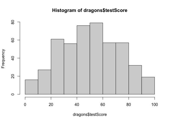
Let’s check distributions. Do test scores and body length measurements look approximately normal?
1
2
#check assumptions: do our continuous variables have approximately normal distributions?
hist(dragons$testScore)
1
hist(dragons$bodyLength)
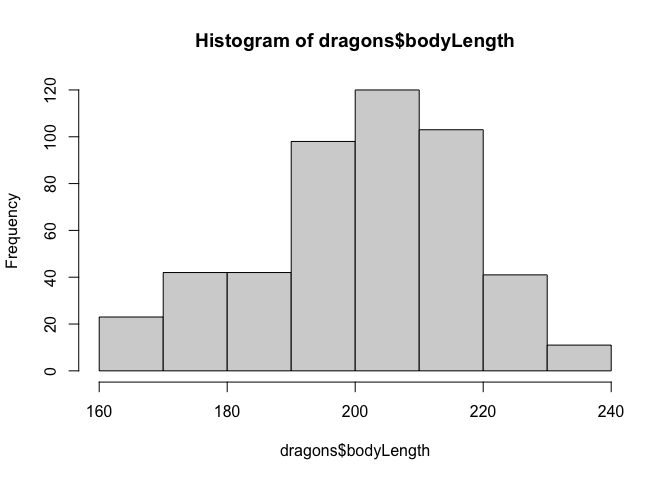
We should mean-center our continuous measure of body length before using it in a model.
1
2
3
4
5
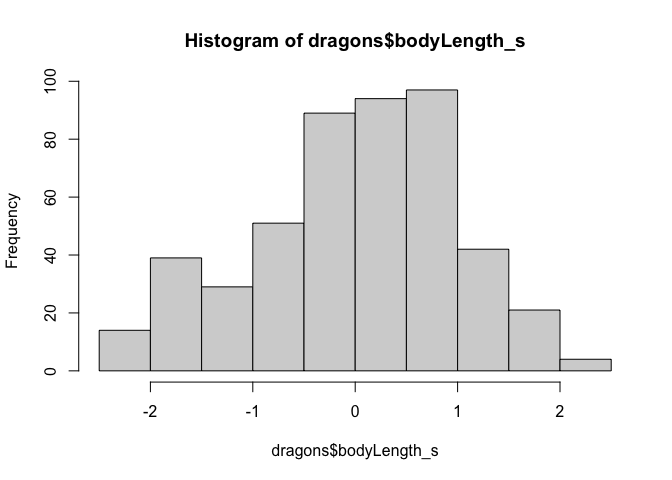
#It is good practice to standardise your explanatory variables before proceeding - you can use scale() to do that:
dragons$bodyLength_s <- scale(dragons$bodyLength)
#Let's look at the histogram again. The scale has changed, so the distribution is now centered around zero.
hist(dragons$bodyLength_s) # seems close to normal distribution - good!
Why do we standardize/mean-center variables? Should we also standardize testScore? Why or why not?
Linear Regression
Okay, let’s start fitting some lines! Key Question: Does body
length predict test score?
One way to analyse this data would be to try fitting a linear model to all our data, ignoring all the other variables for now.
This is a “complete pooling” approach, where we “pool” together all the data and ignore the fact that some observations came from specific mountain ranges.
1
2
model <- lm(testScore ~ bodyLength_s, data = dragons)
summary(model)
1
2
3
4
5
6
7
8
9
10
11
12
13
14
15
16
17
18
##
## Call:
## lm(formula = testScore ~ bodyLength_s, data = dragons)
##
## Residuals:
##     Min      1Q  Median      3Q     Max
## -56.962 -16.411  -0.783  15.193  55.200
##
## Coefficients:
##              Estimate Std. Error t value            Pr(>|t|)
## (Intercept)   50.3860     0.9676  52.072 <0.0000000000000002 ***
## bodyLength_s   8.9956     0.9686   9.287 <0.0000000000000002 ***
## ---
## Signif. codes:  0 '***' 0.001 '**' 0.01 '*' 0.05 '.' 0.1 ' ' 1
##
## Residual standard error: 21.2 on 478 degrees of freedom
## Multiple R-squared:  0.1529, Adjusted R-squared:  0.1511
## F-statistic: 86.25 on 1 and 478 DF,  p-value: < 0.00000000000000022
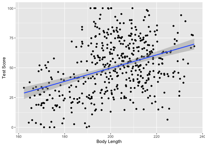
Incredible! It’s super significant! We’re gonna publish in Nature Dragonology!
Let’s plot the data with ggplot2 to see the correlation.
1
2
3
4
5
ggplot(dragons, aes(x = bodyLength, y = testScore)) +
  geom_point()+
  geom_smooth(method = "lm") +
  xlab("Body Length")+
  ylab("Test Score")
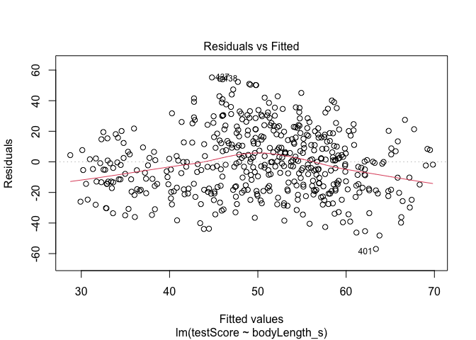
Wait, but we need to check assumptions!
1
2
#Let's plot the residuals from this model. Ideally, the red line should be flat.
plot(model, which = 1)  # not perfect, but looks alright
1
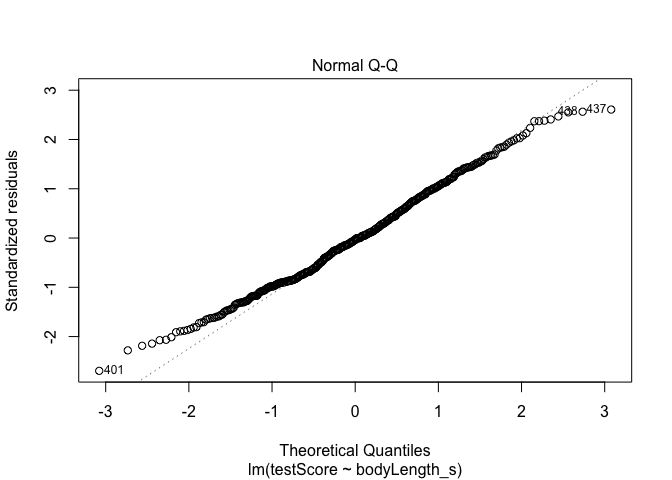
2
#Have a quick look at the qqplot too - point should ideally fall onto the diagonal dashed line
plot(model, which = 2) # a bit off at the extremes, but that's often the case; again doesn't look too bad
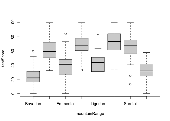
But linear models also assume that observations are INDEPENDENT. Uh oh.
We collected multiple samples from eight mountain ranges. It’s perfectly plausible that the data from within each mountain range are more similar to each other than the data from different mountain ranges - they are correlated. This could be a problem.
1
2
#Have a look at the data to see if above is true
boxplot(testScore ~ mountainRange, data = dragons)  # certainly looks like something is going on here
1
2
3
4
5
#We could also plot it colouring points by mountain range
ggplot(dragons, aes(x = bodyLength, y = testScore, colour = mountainRange))+
  geom_point(size = 2)+
  theme_classic()+
  theme(legend.position = "none")
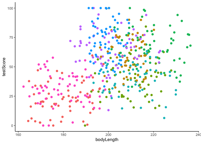
Clearly, there is structured variance in our data that has something to do with the mountain range where we found the dragons.
How do we deal with this variance? We could run many separate analyses and fit a regression for each of the mountain ranges. Let’s check what it would look like if we fit a separate regression line for each mountain range.
1
2
3
4
5
6
7
#Lets have a quick look at the data split by mountain range
#We use the facet_wrap to do that
ggplot(data = dragons, aes(x = bodyLength_s, y = testScore)) +
  stat_smooth(method = "lm", se = FALSE, size = 1.5) +
  geom_point() +
  facet_wrap(.~mountainRange) +
  xlab("length") + ylab("test score")
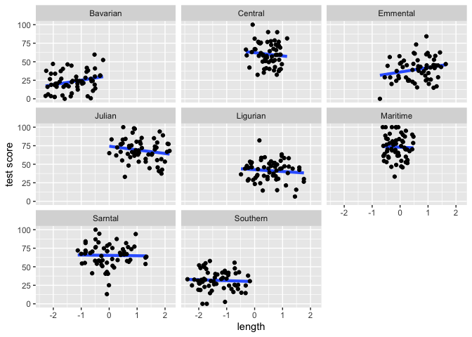
From the above plots it looks like our mountain ranges vary both in the dragon body length and in their test scores. This confirms that our observations from within each of the ranges aren’t independent. We can’t ignore that.
So, what if we estimate the effect of bodyLength on testScore for each range independently?
This would be a no-pooling approach: fitting a separate line for each mountain range, and ignoring our group-level information. This approach treats each group of observations (in this case, mountainRange, but could be participants in other datasets) totally independently.
1
2
3
4
5
6
7
8
df_no_pooling <- lmList(testScore ~ bodyLength_s | mountainRange, data = dragons) %>%
  coef() %>%
  # Mountain Range IDs are stored as row-names above. Let's also add a column to label them.
  rownames_to_column("mountainRange") %>%
  rename(Intercept = `(Intercept)`, Slope_length = bodyLength_s) %>%
  add_column(Model = "No pooling")

head(df_no_pooling)
1
2
3
4
5
6
7
##   mountainRange Intercept Slope_length      Model
## 1      Bavarian  31.20839     6.123797 No pooling
## 2       Central  62.18653    -4.320506 No pooling
## 3      Emmental  36.07089     6.027930 No pooling
## 4        Julian  74.30562    -4.909633 No pooling
## 5      Ligurian  42.67941    -2.475646 No pooling
## 6      Maritime  73.01376    -1.785289 No pooling
Check out the variation in the intercepts and slopes when we fit a separate model for each mountain range.
How do our estimates compare for the complete pooling vs. no pooling methods?
1
2
3
4
5
6
7
8
9
#First, let's grab the coefficients from the first model we fit (the simple linear regression that ignores mountain range information)
df_pooled <- tibble(
  Model = "Complete pooling",
  mountainRange = unique(dragons$mountainRange),
  Intercept = coef(model)[1],
  Slope_length = coef(model)[2])

#You can see that this just copies the same group-level line estimate for every mountain range
head(df_pooled)
1
2
3
4
5
6
7
8
9
## # A tibble: 6 x 4
##   Model            mountainRange Intercept Slope_length
##   <chr>            <chr>             <dbl>        <dbl>
## 1 Complete pooling Bavarian           50.4         9.00
## 2 Complete pooling Central            50.4         9.00
## 3 Complete pooling Emmental           50.4         9.00
## 4 Complete pooling Julian             50.4         9.00
## 5 Complete pooling Ligurian           50.4         9.00
## 6 Complete pooling Maritime           50.4         9.00
1
2
3
4
#Let's combine this with the estimates from the no-pooling approach
df_models <- bind_rows(df_pooled, df_no_pooling) %>%
  left_join(dragons, by = "mountainRange")
head(df_models)
1
2
3
4
5
6
7
8
9
10
## # A tibble: 6 x 10
##   Model mountainRange Intercept Slope_length testScore bodyLength color diet
##   <chr> <chr>             <dbl>        <dbl>     <dbl>      <dbl> <chr> <chr>
## 1 Comp… Bavarian           50.4         9.00     0           176. Blue  Carn…
## 2 Comp… Bavarian           50.4         9.00     0.743       191. Blue  Carn…
## 3 Comp… Bavarian           50.4         9.00     2.50        170. Blue  Carn…
## 4 Comp… Bavarian           50.4         9.00     3.38        189. Blue  Carn…
## 5 Comp… Bavarian           50.4         9.00     4.58        174. Blue  Carn…
## 6 Comp… Bavarian           50.4         9.00    12.5         183. Blue  Carn…
## # … with 2 more variables: breathesFire <int>, bodyLength_s[,1] <dbl>
1
2
3
4
5
#Let's plot the two linear estimates for each mountain range
ggplot(data = df_models, aes (x = bodyLength_s, y = testScore)) +
  geom_point() +
  geom_abline(aes(intercept = Intercept, slope = Slope_length, color = Model), size = 1)+
  facet_wrap(.~mountainRange)
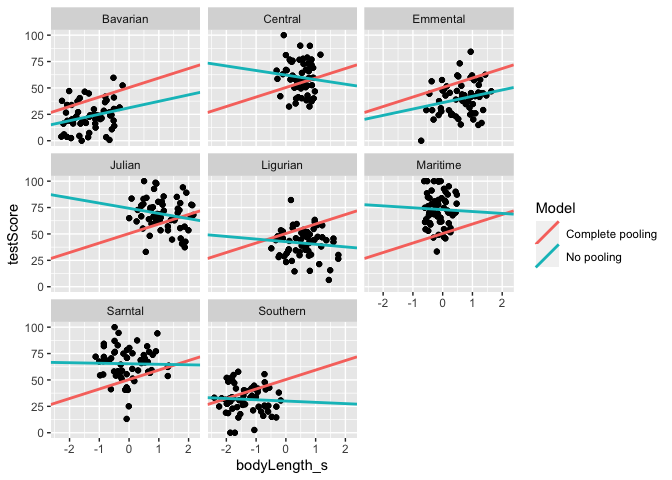
We got very different estimates from the two different approaches. Is there a happy medium?
Linear Mixed Effects Regression
Mountain range clearly introduces a structured source of variance
in our data. We need to control for that variation if we want to
understand whether body length really predicts test scores.
But it doesn’t really make sense to estimate the effect for each mountain range separately. Shouldn’t we use the full power of our whole dataset?
Mixed effects regression is a compromise: Partial pooling! We can let
each mountain range have it’s own regression line, but make an informed
guess about that line based on the group-level estimates This is
especially useful when some groups/participants have incomplete data.
Should Mountain Range be a FIXED or RANDOM effect?
We could consider it a FIXED EFFECT if we were interested in testing the hypothesis that location of residence influences test scores– but that’s not our research question! This is just annoying noise that limits our ability to test the relationship between body length and test scores. So, we need to account for structured variance among mountain ranges by modelling it as a RANDOM EFFECT.
1
2
3
4
5
6
7
#let's fit our first mixed model!
mixed_model <- lmer(testScore ~ bodyLength_s + (1+bodyLength_s|mountainRange), data = dragons)

#note that you might get a "singular fit" warning --> In this case, it's because the data are made-up and we've got some weird correlations in our random effects structure. If you get this with real data, it's not necessarily terrible, but it indicates that you should check for either very high or very low covariance, and try modifying your random effects structure.

#what's the verdict?
summary(mixed_model)
1
2
3
4
5
6
7
8
9
10
11
12
13
14
15
16
17
18
19
20
21
22
23
24
25
26
27
28
29
30
## Linear mixed model fit by REML. t-tests use Satterthwaite's method [
## lmerModLmerTest]
## Formula: testScore ~ bodyLength_s + (1 + bodyLength_s | mountainRange)
##    Data: dragons
##
## REML criterion at convergence: 3980.5
##
## Scaled residuals:
##     Min      1Q  Median      3Q     Max
## -3.5004 -0.6683  0.0207  0.6592  2.9449
##
## Random effects:
##  Groups        Name         Variance Std.Dev. Corr
##  mountainRange (Intercept)  324.102  18.003
##                bodyLength_s   9.905   3.147   -1.00
##  Residual                   221.578  14.885
## Number of obs: 480, groups:  mountainRange, 8
##
## Fixed effects:
##              Estimate Std. Error       df t value  Pr(>|t|)
## (Intercept)  51.75302    6.40349  6.91037   8.082 0.0000916 ***
## bodyLength_s -0.03326    1.68317 10.22337  -0.020     0.985
## ---
## Signif. codes:  0 '***' 0.001 '**' 0.01 '*' 0.05 '.' 0.1 ' ' 1
##
## Correlation of Fixed Effects:
##             (Intr)
## bodyLngth_s -0.674
## convergence code: 0
## boundary (singular) fit: see ?isSingular
Now, let’s see how these lines compare to the no-pooling method.
1
2
3
4
5
6
7
8
9
#save the coefficients from our mixed model
df_partial_pooling <- coef(mixed_model)[["mountainRange"]] %>%
  rownames_to_column("mountainRange") %>%
  as_tibble() %>%
  rename(Intercept = `(Intercept)`, Slope_length = bodyLength_s) %>%
  add_column(Model = "Partial pooling")

#take a peek
head(df_partial_pooling)
1
2
3
4
5
6
7
8
9
## # A tibble: 6 x 4
##   mountainRange Intercept Slope_length Model
##   <chr>             <dbl>        <dbl> <chr>
## 1 Bavarian           28.5         4.02 Partial pooling
## 2 Central            60.8        -1.62 Partial pooling
## 3 Emmental           38.2         2.33 Partial pooling
## 4 Julian             72.7        -3.70 Partial pooling
## 5 Ligurian           40.6         1.92 Partial pooling
## 6 Maritime           72.5        -3.66 Partial pooling
1
2
3
4
5
6
7
8
9
#add these estimates to our dataframe
df_models <- bind_rows(df_pooled, df_no_pooling, df_partial_pooling) %>%
  left_join(dragons, by = "mountainRange")

#Let's plot the three linear estimates for each mountain range
ggplot(data = df_models, aes (x = bodyLength_s, y = testScore)) +
  geom_point() +
  geom_abline(aes(intercept = Intercept, slope = Slope_length, color = Model), size = 1)+
  facet_wrap(.~mountainRange)
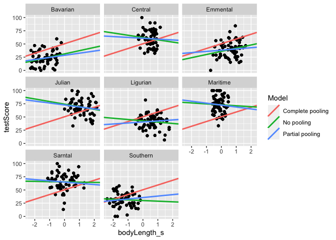
You can see that we get different estimates from all three approaches. Partial pooling yields lines that are tailored to each participant, but still influenced by the pooled group data.
Overall, it looks like when we account for the effect of mountain range, there is no relationship between body length and test scores. Well, so much for our Nature Dragonology paper!
Unless… What about our other variables? Let’s test whether diet is related to test scores instead.
1
2
3
4
mixed_model <- lmer(testScore ~ diet + (1+diet|mountainRange), data = dragons)

#view output
Anova(mixed_model, type=3)
1
2
3
4
5
6
7
8
## Analysis of Deviance Table (Type III Wald chisquare tests)
##
## Response: testScore
##              Chisq Df            Pr(>Chisq)
## (Intercept) 186.75  1 < 0.00000000000000022 ***
## diet        130.55  2 < 0.00000000000000022 ***
## ---
## Signif. codes:  0 '***' 0.001 '**' 0.01 '*' 0.05 '.' 0.1 ' ' 1
1
summary(mixed_model)
1
2
3
4
5
6
7
8
9
10
11
12
13
14
15
16
17
18
19
20
21
22
23
24
25
26
27
28
29
30
31
32
33
## Linear mixed model fit by REML. t-tests use Satterthwaite's method [
## lmerModLmerTest]
## Formula: testScore ~ diet + (1 + diet | mountainRange)
##    Data: dragons
##
## REML criterion at convergence: 3659.7
##
## Scaled residuals:
##     Min      1Q  Median      3Q     Max
## -2.6961 -0.6041 -0.0268  0.5114  4.5041
##
## Random effects:
##  Groups        Name        Variance Std.Dev. Corr
##  mountainRange (Intercept) 100.765  10.038
##                diet1         6.315   2.513   -0.09
##                diet2        24.214   4.921    0.88 -0.56
##  Residual                  113.340  10.646
## Number of obs: 480, groups:  mountainRange, 8
##
## Fixed effects:
##             Estimate Std. Error      df t value   Pr(>|t|)
## (Intercept)   49.186      3.599   6.749  13.666 0.00000362 ***
## diet1        -15.125      1.332   5.066 -11.354 0.00008537 ***
## diet2         15.028      1.989   6.418   7.554   0.000202 ***
## ---
## Signif. codes:  0 '***' 0.001 '**' 0.01 '*' 0.05 '.' 0.1 ' ' 1
##
## Correlation of Fixed Effects:
##       (Intr) diet1
## diet1 -0.044
## diet2  0.760 -0.573
## convergence code: 0
## boundary (singular) fit: see ?isSingular
What did we find?
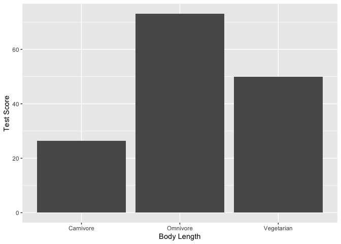
Let’s visualize the effect of diet on test scores.
1
2
3
4
5
#Plot average test score by diet type
ggplot(dragons, aes(x = diet, y = testScore)) +
  geom_bar(stat = "summary")+
  xlab("Body Length")+
  ylab("Test Score")
1
2
3
4
5
6
#Let's also look at the effect across mountain ranges.
ggplot(dragons, aes(x = diet, y = testScore)) +
  geom_bar(stat = "summary")+
  xlab("Body Length")+
  ylab("Test Score") +
  facet_wrap(.~mountainRange)
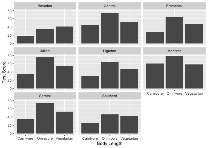
Looks pretty consistent, but there’s obviously still variability between mountains.
Let’s also plot the predicted values from our mixed effects model, so we can control for the effect of mountain range.
1
plot_model(mixed_model, type = "pred", terms = "diet")
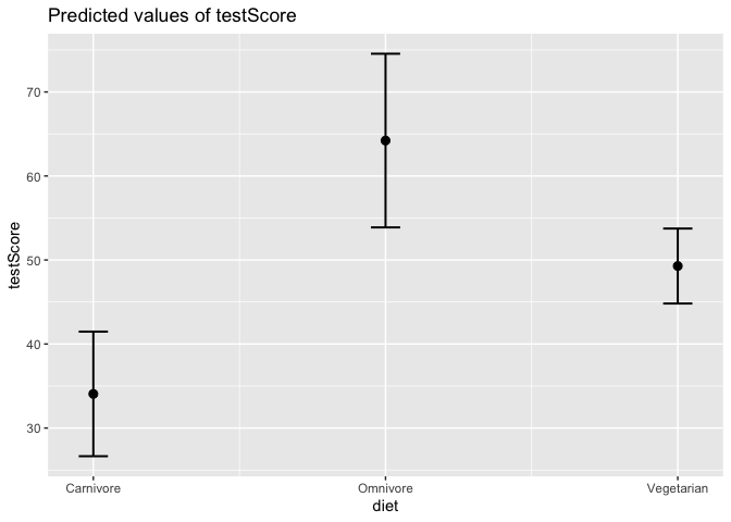
Awesome, we will want to put this finding in our Nature Dragonology paper! Let’s clean up the output.
1
2
#Generate an HTML table with parameter estimates
tab_model(mixed_model, p.val = "satterthwaite", show.df = TRUE, p.style="numeric_stars", show.fstat = TRUE)
| testScore | ||||
|---|---|---|---|---|
| Predictors | Estimates | CI | p | df |
| (Intercept) | 49.19 *** | 42.13 – 56.24 | <0.001 | 8.40 |
| diet1 | -15.13 *** | -17.74 – -12.51 | <0.001 | 11.39 |
| diet2 | 15.03 *** | 11.13 – 18.93 | <0.001 | 50.89 |
| Random Effects | ||||
| σ2 | 113.34 | |||
| τ00 mountainRange | 100.76 | |||
| τ11 mountainRange.diet1 | 6.32 | |||
| τ11 mountainRange.diet2 | 24.21 | |||
| ρ01 | -0.09 | |||
| 0.88 | ||||
| N mountainRange | 8 | |||
| Observations | 480 | |||
| Marginal R2 / Conditional R2 | 0.575 / NA | |||
| * p<0.05 ** p<0.01 *** p<0.001 | ||||
What if we want to test multiple variables at the same time?
1
2
mixed_model <- lmer(testScore ~ diet * bodyLength_s + (1+diet*bodyLength_s|mountainRange), data = dragons)
Anova(mixed_model, type=3)
1
2
3
4
5
6
7
8
9
10
## Analysis of Deviance Table (Type III Wald chisquare tests)
##
## Response: testScore
##                      Chisq Df          Pr(>Chisq)
## (Intercept)       222.4446  1 <0.0000000000000002 ***
## diet              151.3960  2 <0.0000000000000002 ***
## bodyLength_s        0.0000  1              0.9966
## diet:bodyLength_s   2.3406  2              0.3103
## ---
## Signif. codes:  0 '***' 0.001 '**' 0.01 '*' 0.05 '.' 0.1 ' ' 1
1
summary(mixed_model)
1
2
3
4
5
6
7
8
9
10
11
12
13
14
15
16
17
18
19
20
21
22
23
24
25
26
27
28
29
30
31
32
33
34
35
36
37
38
39
40
41
42
43
44
45
46
47
48
49
50
51
## Linear mixed model fit by REML. t-tests use Satterthwaite's method [
## lmerModLmerTest]
## Formula: testScore ~ diet * bodyLength_s + (1 + diet * bodyLength_s |
##     mountainRange)
##    Data: dragons
##
## REML criterion at convergence: 3651.9
##
## Scaled residuals:
##     Min      1Q  Median      3Q     Max
## -2.8679 -0.5963 -0.0339  0.5147  4.4547
##
## Random effects:
##  Groups        Name               Variance Std.Dev. Corr
##  mountainRange (Intercept)         86.966   9.326
##                diet1                5.002   2.236    0.07
##                diet2               13.235   3.638    0.84 -0.48
##                bodyLength_s         1.920   1.386   -0.84  0.48 -1.00
##                diet1:bodyLength_s   1.092   1.045    0.18  0.99 -0.38  0.37
##                diet2:bodyLength_s   1.070   1.034   -1.00 -0.05 -0.85  0.85
##  Residual                         113.570  10.657
##
##
##
##
##
##
##  -0.17
##
## Number of obs: 480, groups:  mountainRange, 8
##
## Fixed effects:
##                      Estimate Std. Error         df t value   Pr(>|t|)
## (Intercept)         50.052784   3.355964   6.082433  14.915 0.00000509 ***
## diet1              -14.996045   1.287080   2.975401 -11.651    0.00141 **
## diet2               15.484451   1.604576   3.507999   9.650    0.00120 **
## bodyLength_s         0.004232   1.002688  10.623582   0.004    0.99671
## diet1:bodyLength_s  -0.880429   0.934680   8.397553  -0.942    0.37252
## diet2:bodyLength_s   1.502019   0.991514  15.581988   1.515    0.14982
## ---
## Signif. codes:  0 '***' 0.001 '**' 0.01 '*' 0.05 '.' 0.1 ' ' 1
##
## Correlation of Fixed Effects:
##             (Intr) diet1  diet2  bdyLn_ dt1:L_
## diet1        0.075
## diet2        0.659 -0.543
## bodyLngth_s -0.424  0.221 -0.435
## dt1:bdyLng_  0.153  0.409 -0.158  0.059
## dt2:bdyLng_ -0.413 -0.124 -0.323  0.285 -0.500
## convergence code: 0
## boundary (singular) fit: see ?isSingular
Looks like the effect of diet is still significant after we control for body length. We can also see that there’s no significant interaction between diet and body length.
Let’s plot the output again. We can also add multiple terms to our plot of model-predicted values. This is especially helpful when you DO have a significant interaction, and you need to understand why!
1
plot_model(mixed_model, type = "pred", terms = c("diet", "bodyLength_s"))
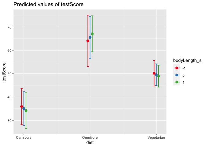
1
2
3
4
#What are the -1, 0, and +1 levels?

#What happens if we swap the order of the terms?
plot_model(mixed_model, type = "pred", terms = c("bodyLength_s", "diet"))
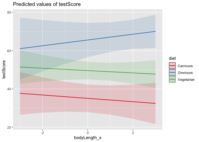
Which version of the plot makes more sense to you?
Your turn! Try modifying the model above to test whether color is related to testScore, and whether color interacts with diet or bodyLength.
1
2
3
4
5
6
7
8
#Build your model here


#View the output of the model here


#Plot your results below:
Mixed Effects Logistic Regression
Okay, let’s test a new question. Test scores are lame. I actually want to know about which dragons breathe fire. This has way more important practical implications, and is more likely to get me grant funding.
Good news: we have data on fire breathing! Bad news: It’s a binary variable, so we need to change our model.
1
2
logit_model <- glmer(breathesFire ~ color + (1+color|mountainRange), data = dragons, family = binomial)
summary(logit_model)
1
2
3
4
5
6
7
8
9
10
11
12
13
14
15
16
17
18
19
20
21
22
23
24
25
26
27
28
29
30
31
32
33
34
## Generalized linear mixed model fit by maximum likelihood (Laplace
##   Approximation) [glmerMod]
##  Family: binomial  ( logit )
## Formula: breathesFire ~ color + (1 + color | mountainRange)
##    Data: dragons
##
##      AIC      BIC   logLik deviance df.resid
##    423.1    460.7   -202.6    405.1      471
##
## Scaled residuals:
##     Min      1Q  Median      3Q     Max
## -3.0000 -0.3083  0.3333  0.3333  4.1246
##
## Random effects:
##  Groups        Name        Variance Std.Dev. Corr
##  mountainRange (Intercept) 0.08865  0.2977
##                color1      0.08866  0.2978   -1.00
##                color2      0.52397  0.7239    0.51 -0.51
## Number of obs: 480, groups:  mountainRange, 8
##
## Fixed effects:
##             Estimate Std. Error z value            Pr(>|z|)
## (Intercept)  0.03662    0.18434   0.199               0.843
## color1       2.16061    0.23902   9.039 <0.0000000000000002 ***
## color2       0.32093    0.31429   1.021               0.307
## ---
## Signif. codes:  0 '***' 0.001 '**' 0.01 '*' 0.05 '.' 0.1 ' ' 1
##
## Correlation of Fixed Effects:
##        (Intr) color1
## color1 -0.246
## color2  0.019 -0.323
## convergence code: 0
## boundary (singular) fit: see ?isSingular
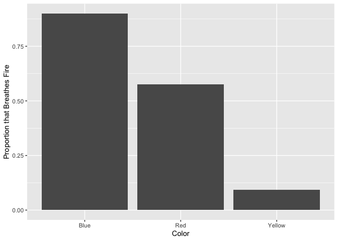
Let’s plot the proportion of dragons that breathe fire by color.
1
2
3
4
ggplot(dragons, aes(x = color, y = breathesFire)) +
  geom_bar(stat = "summary")+
  xlab("Color") +
  ylab("Proportion that Breathes Fire")
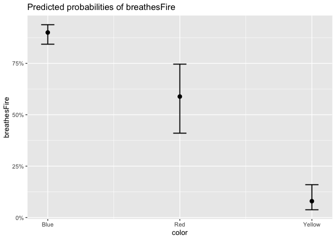
Let’s also get the predicted values from our mixed effects model, so we can control for the effect of mountain range.
1
plot_model(logit_model, type = "pred", terms = "color")
1
2
#generate an HTML table with parameter estimates
tab_model(logit_model, show.df = TRUE, p.style="numeric_stars", show.fstat = TRUE)
| breathesFire | ||||
|---|---|---|---|---|
| Predictors | Odds Ratios | CI | p | df |
| (Intercept) | 1.04 | 0.72 – 1.49 | 0.843 | Inf |
| color1 | 8.68 *** | 5.43 – 13.86 | <0.001 | Inf |
| color2 | 1.38 | 0.74 – 2.55 | 0.307 | Inf |
| Random Effects | ||||
| σ2 | 3.29 | |||
| τ00 mountainRange | 0.09 | |||
| τ11 mountainRange.color1 | 0.09 | |||
| τ11 mountainRange.color2 | 0.52 | |||
| ρ01 | -1.00 | |||
| 0.51 | ||||
| ICC | 0.11 | |||
| N mountainRange | 8 | |||
| Observations | 480 | |||
| Marginal R2 / Conditional R2 | 0.496 / 0.553 | |||
| * p<0.05 ** p<0.01 *** p<0.001 | ||||
Your turn! Test whether other variables predict breathesFire.
1
2
3
4
5
#Build your model here:


#Plot your results:
Convergence
Some parting tips and tricks:
If you ever encounter an error message about “convergence failure,” you cannot trust the results of your model! What can you do to fix this error?
First, check that your continuous predictor variables are all scaled/mean-centered.
Make sure your random effects structure is correct. Are you accidentally specifying random effects that don’t make sense for the data? For example, you can never use a between-subs variable as a random slope when you have a random intercept term for subjects. That wouldn’t make sense, because you only have one observation per subject.
You can also try simplifying your random effects structure. You can start with a maximal model (all possible random slopes and intercepts), and then incrementally prune away random effects terms (starting with interactions in random slopes, etc.) until you achieve convergence. You can also formally compare model fits to determine the optimal random effects structure that is justified by the data.
Lastly, you may need to change the settings of your model and increase
the maximum number of iterations. Adding the following code within your
lmer() call may help: control=lmerControl(optimizer=“bobyqa”, optCtrl=list(maxfun=10e4))
Check that your random effects variables have at least 5 levels each (e.g., 5+ subjects, 5+ observation sites, etc.)
If these tricks still doesn’t help, it may be that you just don’t have enough data to fit the model appropriately! You must have enough observations for every combination of fixed and random effect in order to estimate the variance. You may need to get more data, or prune your model to remove interaction terms that may be causing the problem. For example, a 2x2 interaction term between factor variables assumes that you have data for all 4 possible combinations. If you add more and more interactions, you’re creating a lot of cells that you need to fill.
1
hist(dragons$bodyLength)
Why do we standardize/mean-center variables? Should we also standardize testScore? Why or why not?
1
2
#Have a quick look at the  qqplot too - point should ideally fall onto the diagonal dashed line
plot(model, which = 2)  # a bit off at the extremes, but that's often the case; again doesn't look too bad
1
2
3
4
5
#We could also plot it colouring points by mountain range
ggplot(dragons, aes(x = bodyLength, y = testScore, colour = mountainRange))+
  geom_point(size = 2)+
  theme_classic()+
  theme(legend.position = "none")
Clearly, there is structured variance in our data that has something to do with the mountain range where we found the dragons.
From the above plots it looks like our mountain ranges vary both in the dragon body length and in their test scores. This confirms that our observations from within each of the ranges aren’t independent. We can’t ignore that.
We got very different estimates from the two different approaches. Is there a happy medium?
You can see that we get different estimates from all three approaches. Partial pooling yields lines that are tailored to each participant, but still influenced by the pooled group data.
1
2
3
4
5
6
#Let's also look at the effect across mountain ranges.
ggplot(dragons, aes(x = diet, y = testScore)) +
  geom_bar(stat = "summary")+
  xlab("Body Length")+
  ylab("Test Score") +
  facet_wrap(.~mountainRange)
Looks pretty consistent, but there’s obviously still variability between mountains.
1
2
3
4
#What are the -1, 0, and +1 levels?

#What happens if we swap the order of the terms?
plot_model(mixed_model, type = "pred", terms = c("bodyLength_s", "diet"))
Which version of the plot makes more sense to you?
1
2
#generate an HTML table with parameter estimates
tab_model(logit_model, show.df = TRUE, p.style="numeric_stars", show.fstat = TRUE)
| breathesFire | ||||
|---|---|---|---|---|
| Predictors | Odds Ratios | CI | p | df |
| (Intercept) | 1.04 | 0.72 – 1.49 | 0.843 | Inf |
| color1 | 8.68 *** | 5.43 – 13.86 | <0.001 | Inf |
| color2 | 1.38 | 0.74 – 2.55 | 0.307 | Inf |
| Random Effects | ||||
| σ2 | 3.29 | |||
| τ00 mountainRange | 0.09 | |||
| τ11 mountainRange.color1 | 0.09 | |||
| τ11 mountainRange.color2 | 0.52 | |||
| ρ01 | -1.00 | |||
| 0.51 | ||||
| ICC | 0.11 | |||
| N mountainRange | 8 | |||
| Observations | 480 | |||
| Marginal R2 / Conditional R2 | 0.496 / 0.553 | |||
| * p<0.05 ** p<0.01 *** p<0.001 | ||||