A summary and some questions for group discussion.

Overview

• Background
• Arguments supporting nonlinear approaches
• Reasons to prefer linear regression analysis (for estimating causal effects on binary outcomes)
• Analytical evidence
• Simulation evidence
• Empirical evidence
• Summary and conclusion

Background

A lot of psychology research uses binary dependent (or outcome) variables, such that responses are either 0 or 1. The paper lists social psych examples, but pretty much anytime a cog psych experiment measures accuracy on a trial-by-trial basis, it’s done using a binary outcome. It’s basically dogma that when you have a binary outcome, you use a logistic regression (or logit model) rather than a linear regression (or linear model; which is used for continuous variables). Some people use probit models to analyze binary outcomes, but I’m of the understanding that it’s more commonly used when your outcome is ordinal but not quite continuous/linear (e.g., confidence ratings on a scale of 1-4). But it’s been argued that even 7-point Likert scales commonly treated as continuous in psych research should be analyzed with probit models.

The difference between linear, logit, and probit models is the link function. Link functions transform the outcome variable to a continuous scale, allowing the predictors and response to be modeled with linear regression. But when you move to the other side of the equation (i.e., applying the inverse link function), then your coefficients are transformed to the outcome scale of interest. The inverse logit takes a continuous number (log odds) and converts it to a probability. The inverse probit function is just the density function of a normal distribution – it converts a normally distributed latent variable to a probability.^{thanks Kevin}

Arguments supporting nonlinear approaches (or, the standard view)

1. Nonlinear models are necessary if your goal is prediction

The most popular argument for using these models for binary outcomes is that they constrain parameter estimates between 0 and 1. If a researcher is interested in predicting the likelihood that someone does something, it helps to have coefficients that are directly related to the behavior of interest.

2. Predictions outside the interval unit yields biased and inconsistent parameter estimates

Horrace and Oaxaca (2008) showed that bias and inconsistenty of an estimator increase with the proportion of predicted probabilities that fall outside of the interval unit.

3. Binary outcomes violate the assumption of homoskedasticity

That is, the variance of the error term for binary outcomes is unequal for all values of X. This biases the standard errors of ordinary least squares estimates by placing too much weight on some portion of the data.

Just how relevant are these concerns for psychology research?

Spoiler: not super relevant

1. Psychology research, Gomila argues, is mainly focused on estimating causal effects, or identifying mechanisms that cause particular behaviors or mental processes. The question then becomes to what extent do out-of-bound predictions bias estimates of causal effects?

2. Causal effects are probed via experiments where participants are randomly assigned to a treatment vs. control condition. If you regress a binary treatment onto a binary outcome, it’s impossible for estimates to be out-of-bound or biased. (so the answer to the above is no)

3. This holds when you have covariates that are discrete and take on a few values. In fact, when a model is saturated (the dependent variable is regressed on a set of binary variables & categorical variables with more than 2 values are dummy coded) or fully interacts with binary covariates, the underlying structure of the model is inherently linear so estimates will unbiased, consistent, and never out-of-bounds.

4. However, if you have continuous covariates, then the underlying model structure is nonlinear. Linear regression will not do a good job approximating this model. But Gomila adds that it’s unclear that logit or probit constitute correct approximations of this model.

5. Re violation of homoskedasticity, Angrist and Pischke (2009) have argued that most real-world variables violate this assumption anyway, regardless of whether they are binary or continuous. Since heteroskedasticity is derives from how you calculate standard errors, you can do so in such a way that is heteroskedascity-robust.

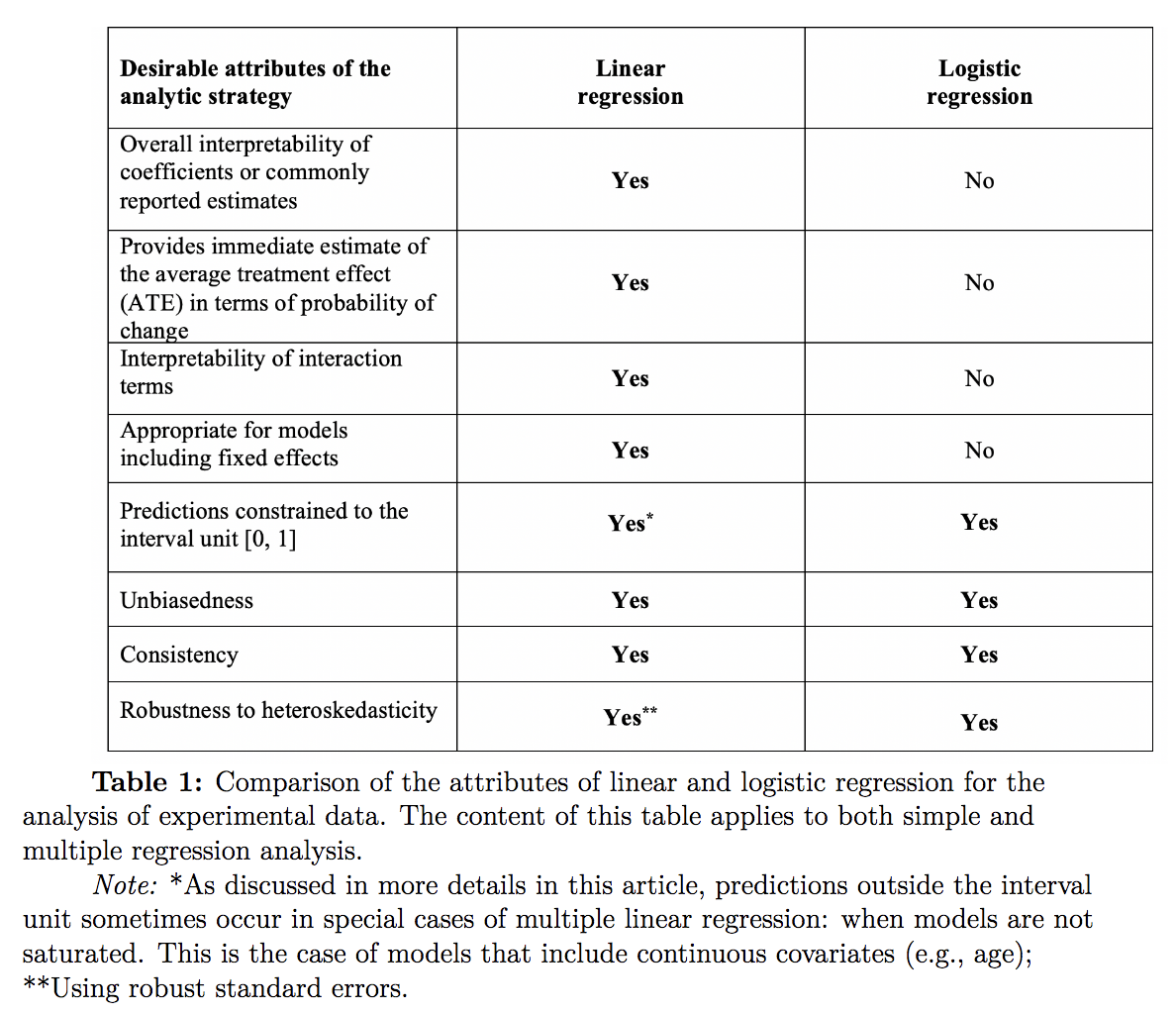
Reasons to prefer linear regression

1. Target estimands and interpretability

The coefficients of nonlinear models are never directly interpretable. But even after transformation (e.g., going from log odds to odds ratios), most researchers don’t have a clear sense of precisely what an odds ratio represents. Or if they do, it is cumbersome and difficult to communicate effectively. Gomila argues that this shifts the focus of analyses to statistical significance instead of effect size, which is a more robust and informative metric of your target estimand (or quantity of interest).

When your target estimand is the causal effect of a treatment on an outcome variable, the coefficients obtained via linear regression are directly interpretable as changes in the percentage points of the probability of observing the outcome. Let’s look at equation 3 to see how this is true:

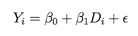
where i denotes individuals and D denotes treatment. In this setup, when you are regressing a binary outcome onto a binary treatment, the average treatment effect is equal to B_i directly expressed in terms of probabilities. Gomila does not give any more detail than this, so someone with a stronger math background than me should explain to us why this is true.

He says this later on but I think it fits well here. Not only are odds ratios difficult to interpret (a ratio of ratios??), but the relevance of effects expressed in odds ratios is conditional on the mean of the dependent variable for the control group. So an odds ratio of X could correspond to a very small effect if the mean of the dependent variable of the control group is tiny, or to a larger effect if the mean of the dependent variable of the control group is larger. This means that the same odds ratio can translate into different Cohen’s d values depending on the mean of the dependent variable of the control condition.

2. (Mis)conception of interaction effects in nonlinear models

In nonlinear models, interaction effects are conditional on other independent variables, thus leading to covariance of the size & sign of an interaction effect with the values of other independent variables. So the sign of an interaction’s coefficient doesn’t necessarily reflect the actual sign of the interaction, and the statistical significance is contingent on whether the interaction is conceptualized in terms of probabilities, log odds, or odds ratios. Thus, misinterpretation of interactions runs abound among users of logistic regression.

Author notes: Is this news to anyone else? Does someone who knows more want to tell us why this is true only for nonlinear models?

3. Nonlinear models don’t perform well in the presence of fixed effects

Because logit models drop all observations that don’t vary in the outcome variable, using a fixed effects structure can lead to just as much bias as models that ignore the hierarchical structure of the data. But the opposite is true for linear regression–its performance vs. nonlinear models increases with the number of fixed effects.

Author notes: I have some questions. 1) I thought it was random effects that acocunt for hierarchical structure. 2) What’s the difference (in implementation) between a fixed effect and a treatment variable? Assuming Gomila & I are talking about the same thing when we say fixed effect, then to my understanding you would program a fixed effect and a treatment effect identically in lmer as outcome ~ independent variable(s).

Analytical evidence of the unbiasedness and consistency of the OLS estimator

The Neyman-Rubin Causal Model

This approach estimates causal effects in terms of counterfactuals (i.e., potential outcomes). This model accounts for the facts (1) that the effect of treatment can vary between individuals and (2) that you only observe behavior of an individual in one of the two conditions by comparing treated and untreated individuals and then adding in a bias term.

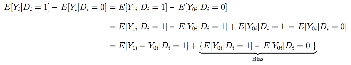
where Y_1i is the outcome if the individual is treated, Y_0i is the outcome if the individual is not treated, and D_i is the treatment.

The average causal effect of the treatment in experiments is unbiased and consistent

D_i and Y_0i are independent in experimental designs. Thus, we can express the average treatment effect (tau_i) as

This is usually referred to as the unconditional causal effect of the treatment, and Y_i being binary has no implications for that; i.e., the outcome is unbiased and consistent.

Comparison of linear and logistic regression results using simulation

Simulation of population data

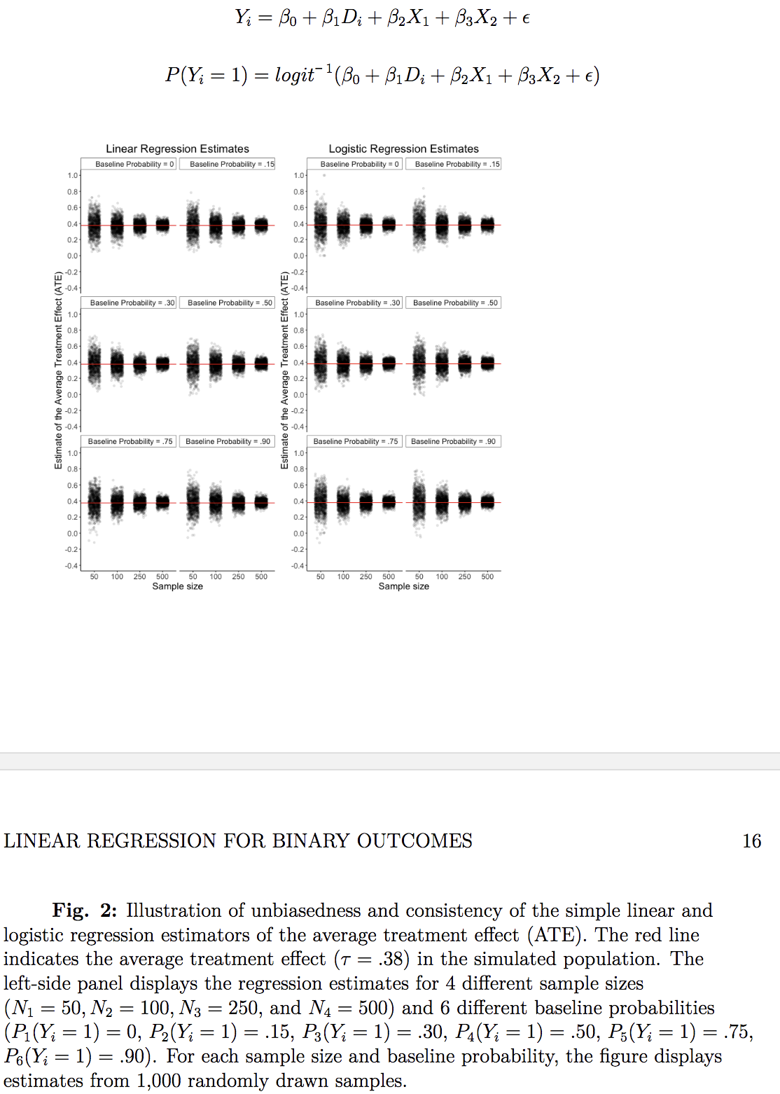
There are 6 different binary variables for each the control (Y_01i, Y_02i, … , Y_06i) and treatment (Y_11i, Y_12i, … , Y_16i) conditions. The potential outcomes for each of these variables has a different baseline probability of success varying from 0 to 0.9. There are two covariates: X₁, a binary variable indicating college degree, and X₂, a discrete variable indicating religiosity on a 5-point scale.

Estimation of the average treatment effect in experiments

The randomized treatment has an average effect=.08, or 8 percentage points. After drawing several random samples & randomly assigning individuals to groups, you see that you obtain the same result using the linear and logistic regression models.

Estimation of the average treatment effect in quasi-experiments

Now we’re including our two covariates. The potential outcomes for both the treatment and control conditions were generated from a logit model that uses both covariates. Then random sample, random assign, and voila:

Comparison of linear and logistic regression results using existing data

Dataset

A field experiment examining the impact of an anti-conflict intervention in 56 New Jersey middle schools (n=24,191 students). Schools were assigned to blocks of 2 before being randomly assigned, within their block, to a treatment or control condition. The intervention lasted a year.

Selection of the variables and analytic strategy

Gomila chose 12 different binary variables with varying distributions. He compares the regression coefficients reported from the researcher to the probabilities derived from linear models, and does this for both pooled & nested effect structures.

Results

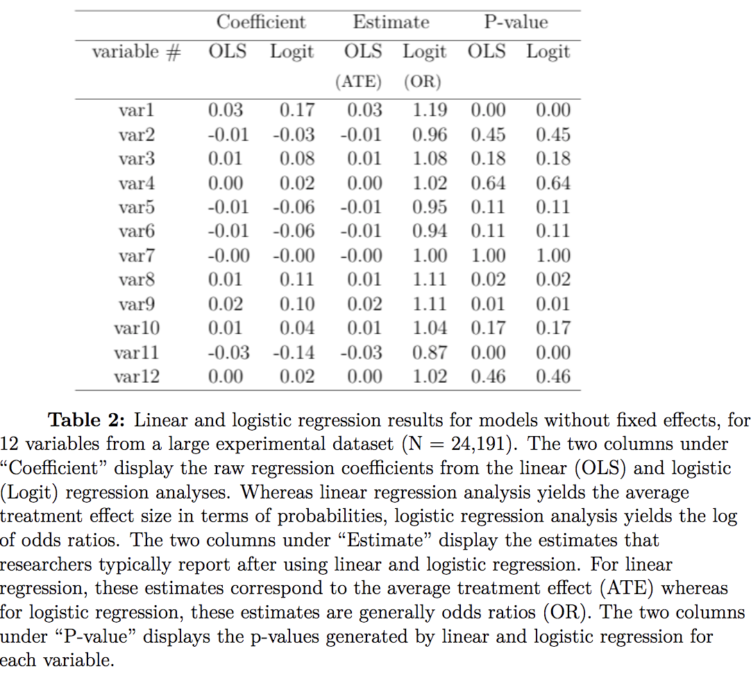
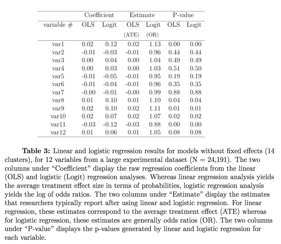
There is hardly a difference between linear and logit models. However, the equal performance on this dataset might not generalize to others. This one has small clusters and a large N, and the n in each cluster explains the effectiveness of logistic regression – logit performance can be expected to decrease as the ratio of observations to clusters decreases.

Summary & conclusions

Basically just

Given the similarity in performance but disparity in interpretability, linear models for binary outcomes are almost always preferred to nonlinear models. The only exception is when the model is not saturated, e.g., has continuous covariates. Gomila suggests that in this case a linear model is accompanied by a sensitivity analysis that analyzes the data with nonlinear models (logit/probit) or clustering methods (Bernoulli mixture models) to assess the robustness of the estimates.