
Reinforcement Learning

Our Scenario
In this workshop we will simulate an agent solving a 2-armed bandit
task. Each arm can give a reward (reward = 1) or not (reward = 0).
Arm 1 will give a reward 70% of the time and Arm 2 will only
give a reward 30% of the time, but our agent doesn’t know that. By
the end of the exercise, our agent will hopefully choose Arm 1 most
of the time, and you will understand the logic and computations that
drive this learning.
Coding:
We will be programming our agent in R. We will start by initializing a few variables that describe our scenario. We can change these later to visualize different scenarios.
1
2
3
4
#variable declaration
nArms <- 2 #number of bandit arms
banditArms <- c(1:nArms) #array of length nArms
armRewardProbabilities <- c(0.7, 0.3) #probability of reward for each arm
Step 1: Representing each Arm’s Expected Value
In order for our agent to complete this task, it first needs a way to
represent how valuable it thinks each action is. We operationalize this
with something known as a Q-value. A Q-value is a numerical
representation of the expected average reward of an action. If an action
gives a reward of $0 half of the time and $100 half of the time, its
Q-value is $50, since on average one can expect $50 per action. If
an action gives a reward 0 20% of the time and 1 80% of the time,
its Q-value is 0.8. For now, we will initialize our Q-values for each
arm at 0.5. With time (and rewards), these will be updated to
approximate the correct expected rewards (i.e., the Q-values should
equal to 0.7 and 0.3 eventually since our arms give reward = 1 70%
and 30% of the time.).
Coding:
Let’s initialize our Q-values for each arm at 0.5. We’ll also make a
variable currentQs that will store the Q-values of each arm for the
current trial (since these are needed to determine which arm our agent
will choose).
1
2
3
4
5
6
7
8
9
10
11
Qi <- 0.5 #initial Q value
currentQs <- vector(length = length(banditArms)) #vector that contains the most recent Q-value for each arm

#assign initial Q value to each arm
for (arm in banditArms) {
    currentQs[arm] <- Qi
}

#print Q values
print(noquote("Q values for Arm 1 and Arm 2:"))
print(currentQs)
1
2
## [1] Q values for Arm 1 and Arm 2:
## [1] 0.5 0.5
Step 2: Choosing an action
Next, we need to determine what our action policy is. Given a set of
Q-values, what action do we choose? For this tutorial we are going to
implement something known as a softmax policy, which has a parameter
beta known as the inverse temperature parameter.
Remember, an inverse temperature < 1 means the agent will be increasingly random about which action it picks (ignoring Q-values) and an inverse temperature > 1 means the agent will be in increasingly greedy, predominantly picking the action with the highest current Q-value.
Coding:
We will initialize a beta value (let’s pick 5, a slightly greedier
policy), as well as create a vector choiceProbs that contains the
probabilities of choosing each arm (probabilities will add up to 1). We
will also initialize a vector that contains which action we picked. Once
we have our action probabilities, we will choose one of those action
stochastically (based on the probabilities).
1
2
beta <- 5 #inverse temperature
choiceProbs <- vector(length = length(banditArms)) #contains the probabilities associated with choosing each action
Now, lets caluclate the probability of choosing each arm using the softmax equation:
1
2
3
4
5
6
7
8
9
10
11
12
13
14
15
#calculate sumExp for softmax function
#sumExp is the sum of exponents i.e., what we divide by in our softmax equation
sumExp <- 0
for (arm in banditArms) {
    sumExp <- sumExp + exp(beta * currentQs[arm])
}

#calculate choice probabilities
for (arm in banditArms) {
    choiceProbs[arm] = exp(beta * currentQs[arm]) / sumExp
}

#print probabilities
print(noquote("Probability of choosing Arm 1 and Arm 2:"))
print(choiceProbs)
1
2
## [1] Probability of choosing Arm 1 and Arm 2:
## [1] 0.5 0.5
Since the Q-values are the same (both Qs = 0.5), the arm probabilities
will be the same. Now that we have our probability, lets choose one of
the arms based on those probabilities. Here, it is like flipping a coin.
Sometimes you’ll pick Arm 1, sometimes you’ll pick Arm 2, depending on
the outcome of that coin flip. Try it a few times.
1
2
3
4
5
# choose action given choice probabilities, save in choices vector
choice <- sample(banditArms, size = 1, replace = FALSE, prob = choiceProbs)

#print choice
print(noquote(paste("You picked Arm ",choice,".",sep = "")))
1
## [1] You picked Arm 2.
Step 3: Getting a reward (or not)
Now that we have decided which arm to choose, we go ahead and pull that bandit arm. Depending on the reward probability, we may or may not get a reward. Let’s see what the result is! Feel free to try this a few times as well to confirm that the outcome is stochastic - sometimes you’ll get a reward even if you picked the bad arm (Arm 2), and sometimes you won’t get a reward even if you picked the good arm (Arm 1).
1
2
3
4
5
6
7
8
#given bandit arm choice, get reward outcome (based on armRewardProbabilities)
reward <- rbinom(1,size = 1,prob = armRewardProbabilities[choice])

#print outcome
print(noquote(paste("You picked Arm ",choice,".",sep = "")))
print(noquote(paste("The probability of reward for Arm ",choice," is ",armRewardProbabilities[choice],".", sep = "")))
print(noquote(paste("Your reward outcome is ",reward,".", sep = "")))
print(noquote(ifelse(reward==1,"Hooray!","Too bad :(")))
1
2
3
4
## [1] You picked Arm 2.
## [1] The probability of reward for Arm 2 is 0.3.
## [1] Your reward outcome is 1.
## [1] Hooray!
Step 4: Learning from reward feedback
Whether or not we got a successful reward, we will now update our
initial Q-values based on the reward outcome. If reward = 1, we will
slightly increase the Q-value for the arm we chose. If reward = 0, then
we will slightly decrease the Q-value. How much we update the Q-value up
or down depends on the learning rate parameter alpha.
First, let’s initalize the learning rate to some value. We can play around with this later.
1
alpha <- 0.1 #learning rate
Next, we update the Q-value only for the arm we picked, based on the
reward outcome of choosing that arm. How much we update the Q-value
depends on how high our learning rate alpha is. BE CAREFUL ONLY TO RUN
THIS CELL ONCE.
1
2
3
4
5
6
7
8
9
10
11
12
13
14
15
16
17
18
19
20
21
print(noquote("The old Q values for Arm 1 and Arm 2:"))
print(currentQs)
print(noquote(""))

#caluclate prediction error
predictionError <- reward - currentQs[choice]

print(noquote(paste("You picked Arm ",choice,".",sep = "")))
print(noquote(paste("Our expected value for Arm ", choice, " was ", currentQs[choice], ".", sep="" )))
print(noquote(paste("Instead of ",currentQs[choice], ", our outcome was ",reward,", so our prediction error is ",reward," - ",currentQs[choice]," = ",predictionError, sep="")))
print(noquote(""))
print(noquote(paste("Finally, we multiply our prediction error ",predictionError, " by our learning rate alpha and update our Q value." , sep="")))
print(noquote(paste("New Q-value = Old value (", currentQs[choice], ") + learning rate (", alpha,") * prediction error (", predictionError,")", sep="")))
print(noquote(paste("New Q-value = Old value (", currentQs[choice], ") + ", alpha * (reward - currentQs[choice]), " = ",currentQs[choice] + alpha * (reward - currentQs[choice]), sep="")))
print(noquote(""))

#given reward outcome, update Q values
currentQs[choice] <- currentQs[choice] + alpha * predictionError

print(noquote("Your new updated Q values for Arm 1 and Arm 2:"))
print(currentQs)
1
2
3
4
5
6
7
8
9
10
11
12
13
## [1] The old Q values for Arm 1 and Arm 2:
## [1] 0.5 0.5
## [1]
## [1] You picked Arm 2.
## [1] Our expected value for Arm 2 was 0.5.
## [1] Instead of 0.5, our outcome was 1, so our prediction error is 1 - 0.5 = 0.5
## [1]
## [1] Finally, we multiply our prediction error 0.5 by our learning rate alpha and update our Q value.
## [1] New Q-value = Old value (0.5) + learning rate (0.1) * prediction error (0.5)
## [1] New Q-value = Old value (0.5) + 0.05 = 0.55
## [1]
## [1] Your new updated Q values for Arm 1 and Arm 2:
## [1] 0.50 0.55
Step 5 (AKA Step 1): Given our new Q values, choose a new action, etc
Now that we have new updated Q values, let’s see how the probabilies of choosing each arm have changed!
1
2
3
4
5
6
7
8
9
10
11
12
13
14
15
16
17
18
19
print(noquote("Probability of choosing Arm 1 and Arm 2 from before:"))
print(c(0.5,0.5))
print(noquote(""))

#calculate sumExp for softmax function
#sumExp is the sum of exponents i.e., what we divide by in our softmax equation
sumExp <- 0
for (arm in banditArms) {
    sumExp <- sumExp + exp(beta * currentQs[arm])
}

#calculate choice probabilities
for (arm in banditArms) {
    choiceProbs[arm] = exp(beta * currentQs[arm]) / sumExp
}

#print probabilities
print(noquote("NEW probability of choosing Arm 1 and Arm 2:"))
print(choiceProbs)
1
2
3
4
5
## [1] Probability of choosing Arm 1 and Arm 2 from before:
## [1] 0.5 0.5
## [1]
## [1] NEW probability of choosing Arm 1 and Arm 2:
## [1] 0.4378235 0.5621765
As you can see, we are already more likely to choose the arm that currently has the higher Q-value. This way, we can balance exploration with exploitation. We will continue to pick the worse Arm occassionally, but we’ll also pick the better arm more frequently so that we can maximise reward in the long term.
Simulating a whole process
Now, let’s simulate the agent performing the above steps over and over, 1000 times.
1
2
3
4
5
6
7
8
9
10
11
12
13
14
15
16
17
18
19
20
21
22
23
24
25
26
27
28
29
30
31
32
33
34
35
36
37
38
39
40
41
42
43
44
45
46
47
48
49
50
51
52
53
set.seed(500)

#simulation variables and parameters
nTrials <- 1000
nArms <- 2
banditArms <- c(1:nArms)
armRewardProbabilities <- c(0.7, 0.3) #each arm needs its own reward probability
alpha <- .01 #learning rate
beta <- 5 #inverse temperature
Qi <- 0.5 #initial Q value
currentQs <- vector(length = length(banditArms))
trialQs <- matrix(data = NA, nrow = nTrials, ncol = nArms)
choiceProbs <- vector(length = length(banditArms))
trialChoiceProbs <- matrix(data = NA, nrow = nTrials, ncol = nArms)
choices <- vector(length = nTrials)
rewards <- vector(length = nTrials)

#assign initial Q value
for (arm in banditArms) {
    currentQs[arm] <- Qi
}

for (trial in 1:nTrials) {

    #calculate sumExp for softmax function
    sumExp <- 0
    for (arm in banditArms) {
        sumExp <- sumExp + exp(beta * currentQs[arm])
    }

    #calculate choice probabilities
    for (arm in banditArms) {
        choiceProbs[arm] = exp(beta * currentQs[arm]) / sumExp
    }

    #save choice probabilities in matrix for later visualization
    trialChoiceProbs[trial,] <- choiceProbs

    # choose action given choice probabilities, save in choices vector
    choices[trial] <- sample(banditArms, size = 1, replace = FALSE, prob = choiceProbs)

    #given bandit arm choice, get reward outcome (based on armRewardProbabilities)
    rewards[trial] <- rbinom(1,size = 1,prob = armRewardProbabilities[choices[trial]])

    #given reward outcome, update Q values
    currentQs[choices[trial]] <- currentQs[choices[trial]] + alpha * (rewards[trial] - currentQs[choices[trial]])

    #save Q values in matrix of all Q-values
    trialQs[trial,] <- currentQs
}

#combine choices and rewards into dataframe
df <- data.frame(choices, rewards)
Great job! You should have created a new dataframe df that is filled
with choices and rewards for 1000 trials (or how ever many trials you
specified). Let’s visualize what happened in our simulation by looking
at that dataframe.
1
head(df,100)
1
2
3
4
5
6
7
8
9
10
11
12
13
14
15
16
17
18
19
20
21
22
23
24
25
26
27
28
29
30
31
32
33
34
35
36
37
38
39
40
41
42
43
44
45
46
47
48
49
50
51
52
53
54
55
56
57
58
59
60
61
62
63
64
65
66
67
68
69
70
71
72
73
74
75
76
77
78
79
80
81
82
83
84
85
86
87
88
89
90
91
92
93
94
95
96
97
98
99
100
101
##     choices rewards
## 1         1       0
## 2         1       1
## 3         2       0
## 4         2       1
## 5         1       0
## 6         2       1
## 7         1       1
## 8         1       1
## 9         2       0
## 10        2       0
## 11        1       0
## 12        1       1
## 13        1       0
## 14        2       1
## 15        2       0
## 16        1       1
## 17        2       0
## 18        1       0
## 19        2       0
## 20        2       0
## 21        1       1
## 22        2       0
## 23        2       0
## 24        2       0
## 25        1       1
## 26        1       0
## 27        1       1
## 28        1       1
## 29        1       0
## 30        2       1
## 31        1       0
## 32        2       0
## 33        2       0
## 34        1       1
## 35        1       1
## 36        1       1
## 37        1       1
## 38        2       0
## 39        1       1
## 40        1       1
## 41        1       0
## 42        2       0
## 43        1       0
## 44        2       0
## 45        1       1
## 46        2       1
## 47        1       1
## 48        1       0
## 49        1       1
## 50        1       1
## 51        2       0
## 52        2       0
## 53        2       1
## 54        1       1
## 55        2       0
## 56        2       0
## 57        1       0
## 58        1       0
## 59        1       0
## 60        1       1
## 61        2       1
## 62        1       1
## 63        2       0
## 64        1       0
## 65        2       1
## 66        1       1
## 67        1       1
## 68        1       1
## 69        2       1
## 70        1       1
## 71        1       1
## 72        2       1
## 73        2       1
## 74        1       1
## 75        1       0
## 76        2       1
## 77        1       1
## 78        2       0
## 79        1       1
## 80        1       1
## 81        2       1
## 82        1       1
## 83        2       0
## 84        1       1
## 85        1       1
## 86        1       0
## 87        1       1
## 88        1       1
## 89        2       0
## 90        1       1
## 91        1       1
## 92        2       1
## 93        1       1
## 94        1       1
## 95        2       1
## 96        2       1
## 97        2       0
## 98        1       1
## 99        1       1
## 100       1       1
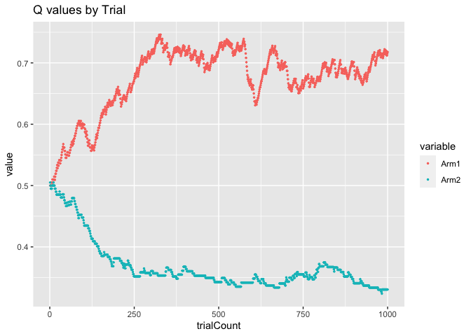
Remember, our goal was for the agent to learn to correctly approximate
the correct reward outcomes for Arm 1 (0.7) and Arm 2 (0.3). Let’s
see what the Q values were estimated at in the last trial.
1
2
print(noquote("The most recent Q-value estimates for Arm 1 and Arm 2:"))
currentQs
1
2
## [1] The most recent Q-value estimates for Arm 1 and Arm 2:
## [1] 0.6617606 0.3559515
Not bad! Our agent’s most recent Q-values were fairly close to the
correct values of 0.7 and 0.3. Of course, the reward outcomes are
probabilistic so we are very unlikely to perfectly estimate the correct
reward probabilities on a given trial. Let’s what the Q-values looked
like over time as the agent performed the task:
1
2
3
4
5
6
7
8
9
10
11
12
13
14
15
16
17
18
19
20
21
library(ggplot2)
library(reshape2)

#turn trialQs matrix into dataframe
Qvalues_df <- as.data.frame(trialQs)

#add column names
for (i in 1:length(Qvalues_df)){
  colnames(Qvalues_df)[i] <- paste("Arm", i, sep="")
}

#add column of trial counts
Qvalues_df$trialCount <- as.numeric(row.names(Qvalues_df))

#turn df into long format for plotting
Qvalues_long <- melt(Qvalues_df, id = "trialCount")

#plot Q values over time
ggplot(data=Qvalues_long, aes(x = trialCount, y = value, color = variable)) +
  geom_point(size = 0.5) +
  ggtitle("Q values by Trial")
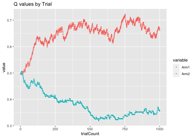
As you can see, over time, the Q-value for Arm 1 came to hover around
the correct value of 0.7 and the Q-value for Arm 2 hovered around the
correct value of 0.3.
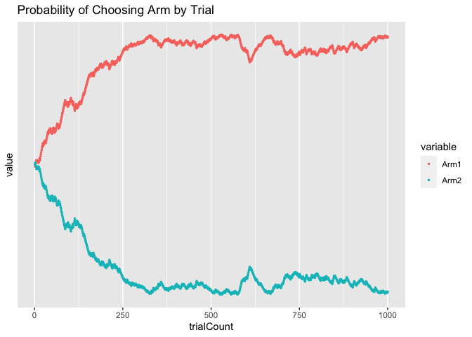
One think you might notice is that the line for the Arm 1 Q-values (red) is much more jagged and changing than the line for Arm 2 (blue), which is fairly smooth. This is because, remember, not only is our agent trying to learn the correct action probabilities, it is also trying to maximize reward. Thus, our agent is actually picking Arm 1 much more frequently than Arm 2 because of it’s higher Q-value. Let’s look at the arm probabilities as they evolved over time.
1
2
3
4
5
6
7
8
9
10
11
12
13
14
15
16
17
18
#turn trial choice probs into dataframe
ChoiceProbs_df <- as.data.frame(trialChoiceProbs)

#add column names
for (i in 1:length(ChoiceProbs_df)){
  colnames(ChoiceProbs_df)[i] <- paste("Arm", i, sep="")
}

#add column of trial counts
ChoiceProbs_df$trialCount <- as.numeric(row.names(ChoiceProbs_df))

#turn df into long format for plotting
ChoiceProbs_long <- melt(ChoiceProbs_df, id = "trialCount")

#plot Q values over time
ggplot(data=ChoiceProbs_long, aes(x = trialCount, y = value, color = variable)) +
  geom_point(size = 0.5) +
  ggtitle("Probability of Choosing Arm by Trial")
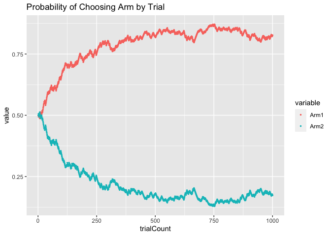
As you can see, initially the agent was equally likely to choose Arm 1 and Arm 2. Over time, however, as the agent learned that Arm 1 had a higher Q-value than Arm 2, it became increasingly likely to choose Arm 1.
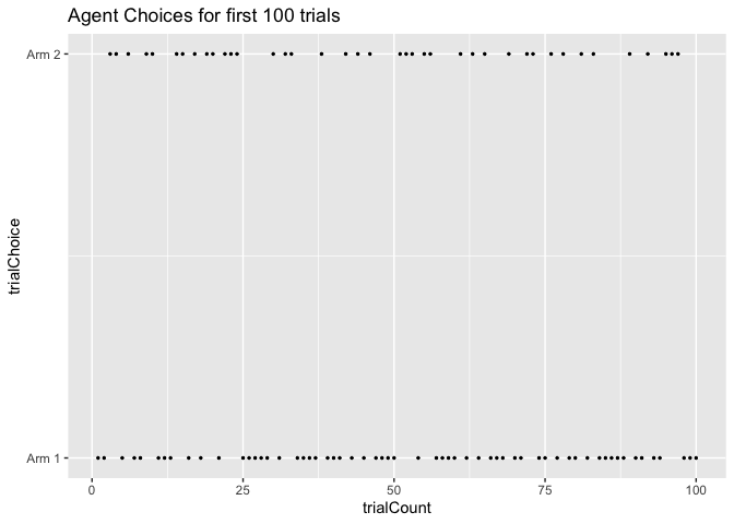
Next, let’s look at the choices the agent actually made. We’ll start by
looking at the choices for the first 100 trials. Since we initialized
both arms Q-values to the same value (0.5), initially our agent was
fairly likely to pick both arms. We can see that below.
1
2
3
4
5
6
7
8
9
10
choice_df <- data.frame(matrix(unlist(choices), nrow=length(choices), byrow=T))

colnames(choice_df)[1] <- "trialChoice"

choice_df$trialCount <- as.numeric(row.names(choice_df))

ggplot(data=choice_df[1:100,], aes(x = trialCount, y = trialChoice)) +
  geom_point(size = 0.5) +
  scale_y_continuous(breaks = 1:2, labels = c("Arm 1","Arm 2")) +
  ggtitle("Agent Choices for first 100 trials")
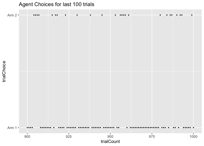
Now let’s look at the last 100 trials instead. By now, the agent has
learned the correct Q-values of each arm and thus is much more likely to
choose Arm 1 (Q-value = 0.7) than Arm 2 (Q-value = 0.3). How much more
likely is determined by our inverse temperature, which determines how
greedy versus exploratory our agent is. We picked a beta of 5, which
is fairly greedy but accurate to how humans usually perform these tasks.
Thus, we can see that in these trials our agent mostly picked Arm 1.
1
2
3
4
ggplot(data=choice_df[900:1000,], aes(x = trialCount, y = trialChoice)) +
  geom_point(size = 0.5) +
  scale_y_continuous(breaks = 1:2, labels = c("Arm 1","Arm 2")) +
  ggtitle("Agent Choices for last 100 trials")
Exercises
Now its your turn! Below is the identical code we just ran. This time, try changing 1 aspect at a time to see what the effect is.
Questions:
-
Leaving everything else constant, what happens when you decrease beta? What happens if you set it to 0?
-
What if beta instead is really large? Try setting it to 100. What happens?
-
What happens if the learning rate is even smaller? Try 0.0001. What if it is bigger? Try 0.2.
-
How does changing the initial Q value affect how quickly the agent starts picking the best action?
1
2
3
4
5
6
7
8
9
10
11
12
13
14
15
16
17
18
19
20
21
22
23
24
25
26
27
28
29
30
31
32
33
34
35
36
37
38
39
40
41
42
43
44
45
46
47
48
49
50
51
52
53
54
55
56
57
58
59
60
61
62
63
64
65
66
67
68
69
70
71
72
73
74
# CHANGE THE VARIABLES BELOW YOURSELF
# vvvvvvvvvvvvvvvvvvvvvvvvvvvvvvvvvvv
nArms <- 2 #<- CHANGE ME
armRewardProbabilities <- c(0.7, 0.3) #probability of reward for each arm <- CHANGE ME
alpha <- .01 #learning rate <- CHANGE ME
beta <- 5 #inverse temperature <- CHANGE ME
Qi <- 0.5 #initial Q value <- CHANGE ME

#simulation variables and parameters
nTrials <- 1000
banditArms <- c(1:nArms)
currentQs <- vector(length = length(banditArms))
trialQs <- matrix(data = NA, nrow = nTrials, ncol = nArms)
choiceProbs <- vector(length = length(banditArms))
trialChoiceProbs <- matrix(data = NA, nrow = nTrials, ncol = nArms)
choices <- vector(length = nTrials)
rewards <- vector(length = nTrials)

#assign initial Q value
for (arm in banditArms) {
    currentQs[arm] <- Qi
}

for (trial in 1:nTrials) {

    #calculate sumExp for softmax function
    sumExp <- 0
    for (arm in banditArms) {
        sumExp <- sumExp + exp(beta * currentQs[arm])
    }

    #calculate choice probabilities
    for (arm in banditArms) {
        choiceProbs[arm] = exp(beta * currentQs[arm]) / sumExp
    }

    #save choice probabilities in matrix for later visualization
    trialChoiceProbs[trial,] <- choiceProbs

    # choose action given choice probabilities, save in choices vector
    choices[trial] <- sample(banditArms, size = 1, replace = FALSE, prob = choiceProbs)

    #given bandit arm choice, get reward outcome (based on armRewardProbabilities)
    rewards[trial] <- rbinom(1,size = 1,prob = armRewardProbabilities[choices[trial]])

    #given reward outcome, update Q values
    currentQs[choices[trial]] <- currentQs[choices[trial]] + alpha * (rewards[trial] - currentQs[choices[trial]])

    #save Q values in matrix of all Q-values
    trialQs[trial,] <- currentQs
}

#combine choices and rewards into dataframe
exercise_df <- data.frame(choices, rewards)

# PLOT Q VALUES OVER TIME
#turn trialQs matrix into dataframe
Qvalues_df <- as.data.frame(trialQs)

#add column names
for (i in 1:length(Qvalues_df)){
  colnames(Qvalues_df)[i] <- paste("Arm", i, sep="")
}

#add column of trial counts
Qvalues_df$trialCount <- as.numeric(row.names(Qvalues_df))

#turn df into long format for plotting
Qvalues_long <- melt(Qvalues_df, id = "trialCount")

#plot Q values over time
ggplot(data=Qvalues_long, aes(x = trialCount, y = value, color = variable)) +
  geom_point(size = 0.5) +
  ggtitle("Q values by Trial")
1
2
3
4
5
6
7
8
9
10
11
12
13
14
15
16
17
18
19
20
# PLOT CHOICE PROBABILITIES
#turn trial choice probs into dataframe
ChoiceProbs_df <- as.data.frame(trialChoiceProbs)

#add column names
for (i in 1:length(ChoiceProbs_df)){
  colnames(ChoiceProbs_df)[i] <- paste("Arm", i, sep="")
}

#add column of trial counts
ChoiceProbs_df$trialCount <- as.numeric(row.names(ChoiceProbs_df))

#turn df into long format for plotting
ChoiceProbs_long <- melt(ChoiceProbs_df, id = "trialCount")

#plot Q values over time
ggplot(data=ChoiceProbs_long, aes(x = trialCount, y = value, color = variable)) +
  geom_point(size = 0.5) +
  scale_y_continuous(breaks = 1:2, labels = c("Arm 1","Arm 2")) +
  ggtitle("Probability of Choosing Arm by Trial")
1
2
3
4
5
6
7
8
9
10
# PLOT FIRST 100 TRIALS
choice_df <- data.frame(matrix(unlist(choices), nrow=length(choices), byrow=T))

colnames(choice_df)[1] <- "trialChoice"

choice_df$trialCount <- as.numeric(row.names(choice_df))

ggplot(data=choice_df[1:100,], aes(x = trialCount, y = trialChoice)) +
  geom_point(size = 0.5) +
  ggtitle("Agent Choices for first 100 trials")

1
2
3
4
5
# AND LAST 100 TRIALS
ggplot(data=choice_df[900:1000,], aes(x = trialCount, y = trialChoice)) +
  geom_point(size = 0.5) +
  scale_y_continuous(breaks = 1:2, labels = c("Arm 1","Arm 2")) +
  ggtitle("Agent Choices for last 100 trials")

Parameter estimation
In the second part of this tutorial, we are going to perform parameter
estimation on our simulated data. Given our data, we would like to
estimate the learning rate alpha and inverse temperature beta that
gave rise to that data. It is important to note that since both our
agent and our bandit arms were stochastic (that is, probabilistic
instead of deterministic), there is necessarily some noise, so our
estimation cannot be perfect. Still, as the number of trials increases
we will be increasingly be able to approximate our learning rate and
inverse temperature.
Our goal in parameter estimation is to find a set of parameter values that maximize the likelihood of the data. In this example, we use stan to do that.
1
2
3
4
5
6
7
8
9
10
11
12
13
14
15
library(rstan)
# create a list object of necessary data vectors
model_data <- list( nArms = length(unique(df$choices)),
                    nTrials = nrow(df),
                    armChoice = df$choices,
                    result = df$rewards)
# fit
simple_RL_model_fit <- stan(
   file = "2020-11-18-simple-RL-model.stan",  # Stan program
   data = model_data,    # named list of data
   chains = 2,             # number of Markov chains
   warmup = 200,          # number of warmup iterations per chain
   iter = 500,            # total number of iterations per chain
   cores = 2
   )
Stan will give you a lot of outputs and warnings, but that doesn’t necessarily mean that sampling failed! A full explanation of stan warnings is outside of the scope of this workshop, but you could check out this brief guide from the stan development team.
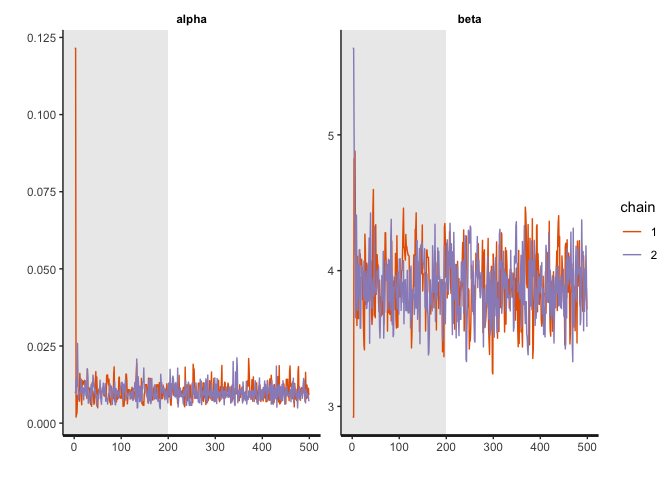
Now, we can check to see how well the sampling worked with some diagnostic plots:
1
traceplot(simple_RL_model_fit, pars = c("alpha","beta"), inc_warmup=TRUE)
1
print(simple_RL_model_fit, pars = c("alpha","beta"))
1
2
3
4
5
6
7
8
9
10
11
12
## Inference for Stan model: 2020-11-18-simple-RL-model.
## 2 chains, each with iter=500; warmup=200; thin=1;
## post-warmup draws per chain=300, total post-warmup draws=600.
##
##       mean se_mean   sd 2.5%  25%  50%  75% 97.5% n_eff Rhat
## alpha 0.01    0.00 0.00 0.01 0.01 0.01 0.01  0.02   541    1
## beta  3.88    0.01 0.22 3.45 3.74 3.88 4.02  4.32   325    1
##
## Samples were drawn using NUTS(diag_e) at Wed Nov 18 10:59:37 2020.
## For each parameter, n_eff is a crude measure of effective sample size,
## and Rhat is the potential scale reduction factor on split chains (at
## convergence, Rhat=1).
What we are looking for is a “hairy caterpillar.” After the warm up period shaded in light grey, the sampled parameter values should stablize.
We can also check the parameter estimates produced by the model. Note that the output is the posterior probability of the parameter rather than a point estimate.
1
stan_hist(simple_RL_model_fit, pars = c("alpha","beta"))
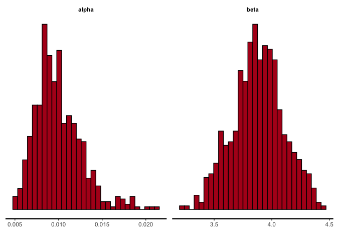
The center of the posterior probability mass should be pretty close to the ground truth parameter values in our data simulation.
Model comparison
There are generally two types of scientific questions we can answer with this kind of modeling approach. The first one is parameter estimation, which we’ve just covered above. By estimating the learning rate, we can answer the question of “How much does a subject update their beliefs based on feedback?” or “How likely is the subject to choose the best option? i.e. How greedy are they versus exploratory?”. The second type of question we can answer is model comparison. Different computational models, in effect, constitute different hypotheses about the learning process that gave rise to the data. These hypotheses may be tested against one another on the basis of their fit to the data. For example, we can ask whether a subject treated positive and negative feedback differently when updating their belief.
Now, we can fit the data to a second model that proposes two learning rates, and see which model produced a better fit in order to adjudicate between the two hypotheses.
1
2
3
4
5
6
7
8
9
# fit
asymmetric_learning_model_fit <- stan(
   file = "2020-11-18-asymmetric-learning-RL-model.stan",  # Stan program
   data = model_data,    # named list of data
   chains = 2,             # number of Markov chains
   warmup = 200,          # number of warmup iterations per chain
   iter = 500,            # total number of iterations per chain
   cores = 2
   )
Now that we have the model estimations from our second model, lets see what it estimates the alpha values to be.
1
2
3
# check parameter estimation
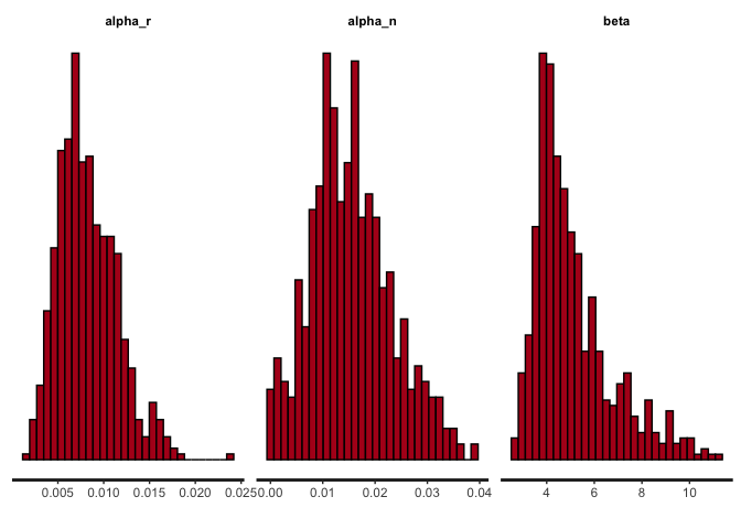
print(asymmetric_learning_model_fit, pars = c("alpha_r","alpha_n","beta"))
stan_hist(asymmetric_learning_model_fit, pars = c("alpha_r","alpha_n","beta"))
1
2
3
4
5
6
7
8
9
10
11
12
13
## Inference for Stan model: 2020-11-18-asymmetric-learning-RL-model.
## 2 chains, each with iter=500; warmup=200; thin=1;
## post-warmup draws per chain=300, total post-warmup draws=600.
##
##         mean se_mean   sd 2.5%  25%  50%  75% 97.5% n_eff Rhat
## alpha_r 0.01    0.00 0.00 0.00 0.01 0.01 0.01  0.02   125 1.01
## alpha_n 0.02    0.00 0.01 0.00 0.01 0.01 0.02  0.03   126 1.01
## beta    5.09    0.17 1.63 3.08 3.94 4.64 5.81  9.35    92 1.01
##
## Samples were drawn using NUTS(diag_e) at Wed Nov 18 11:01:33 2020.
## For each parameter, n_eff is a crude measure of effective sample size,
## and Rhat is the potential scale reduction factor on split chains (at
## convergence, Rhat=1).
The posterior distributions for alpha_r and alpha_n are identical.
This is because we set the same learning rate for rewarded trials and no
reward trials (you could try changing the data simulation code to set
different learning rates and fit the model again).
We will use the loo package, which carries out Pareto smoothed importance-sampling leave-one-out cross-validation, for model comparison:
1
2
3
4
5
6
library(loo)
# Computing PSIS-LOO
loo_simp <- loo(simple_RL_model_fit, save_psis = TRUE)
print(loo_simp)
loo_asym <- loo(asymmetric_learning_model_fit, save_psis = TRUE)
print(loo_asym)
1
2
3
4
5
6
7
8
9
10
11
12
13
14
15
16
17
18
19
20
21
22
23
24
25
26
27
28
29
30
31
32
33
34
##
## Computed from 600 by 1000 log-likelihood matrix
##
##          Estimate   SE
## elpd_loo   -486.7 17.9
## p_loo         2.2  0.1
## looic       973.3 35.7
## ------
## Monte Carlo SE of elpd_loo is NA.
##
## Pareto k diagnostic values:
##                          Count Pct.    Min. n_eff
## (-Inf, 0.5]   (good)     998   99.8%   338
##  (0.5, 0.7]   (ok)         0    0.0%   <NA>
##    (0.7, 1]   (bad)        0    0.0%   <NA>
##    (1, Inf)   (very bad)   2    0.2%   300
## See help('pareto-k-diagnostic') for details.
##
## Computed from 600 by 1000 log-likelihood matrix
##
##          Estimate   SE
## elpd_loo   -486.9 17.7
## p_loo         2.4  0.1
## looic       973.8 35.3
## ------
## Monte Carlo SE of elpd_loo is NA.
##
## Pareto k diagnostic values:
##                          Count Pct.    Min. n_eff
## (-Inf, 0.5]   (good)     998   99.8%   169
##  (0.5, 0.7]   (ok)         0    0.0%   <NA>
##    (0.7, 1]   (bad)        0    0.0%   <NA>
##    (1, Inf)   (very bad)   2    0.2%   300
## See help('pareto-k-diagnostic') for details.
If we had a well-specified model, we would expect the estimated effective number of parameters (p_loo) to be smaller than or similar to the total number of parameters in the model. Pareto k diagnostic values tell us that there are some bad k values, which can make the estimate for the Monte Carlo standard error (SE) of the expected log predictive density (elpd_loo) unreliable (see more information in this loo vignette).
We can use the loo_compare function to compare our two models on expected log predictive density (elpd) for new data
1
2
# Comparing the models on expected log predictive density
loo_compare(loo_simp,loo_asym)
1
2
3
##        elpd_diff se_diff
## model1  0.0       0.0
## model2 -0.2       0.4
The difference in elpd is larger than the estimated standard error of the difference, indicating that the first model with one learning rate is expected to have better predictive performance than the second model with two learning rates. This makes sense, given that the data generating process had only one learning rate for both rewarded and no reward trials.
Exercises
Try simulating data with different payoff probabilities for the two arms, and see how well the model performs.
Try simulating data with a different learning rate or inverse temperature, and see how well the model performs.
Try fitting the model with a different initial Q value by changing the stan file.
As you can see, over time, the Q-value for Arm 1 came to hover around
the correct value of 0.7 and the Q-value for Arm 2 hovered around the
correct value of 0.3.
One think you might notice is that the line for the Arm 1 Q-values (red) is much more jagged and changing than the line for Arm 2 (blue), which is fairly smooth. This is because, remember, not only is our agent trying to learn the correct action probabilities, it is also trying to maximize reward. Thus, our agent is actually picking Arm 1 much more frequently than Arm 2 because of it’s higher Q-value. Let’s look at the arm probabilities as they evolved over time.
1
2
3
4
5
6
7
8
9
10
11
12
13
14
15
16
17
18
#turn trial choice probs into dataframe
ChoiceProbs_df <- as.data.frame(trialChoiceProbs)

#add column names
for (i in 1:length(ChoiceProbs_df)){
  colnames(ChoiceProbs_df)[i] <- paste("Arm", i, sep="")
}

#add column of trial counts
ChoiceProbs_df$trialCount <- as.numeric(row.names(ChoiceProbs_df))

#turn df into long format for plotting
ChoiceProbs_long <- melt(ChoiceProbs_df, id = "trialCount")

#plot Q values over time
ggplot(data=ChoiceProbs_long, aes(x = trialCount, y = value, color = variable)) +
  geom_point(size = 0.5) +
  ggtitle("Probability of Choosing Arm by Trial")
As you can see, initially the agent was equally likely to choose Arm 1 and Arm 2. Over time, however, as the agent learned that Arm 1 had a higher Q-value than Arm 2, it became increasingly likely to choose Arm 1.
Next, let’s look at the choices the agent actually made. We’ll start by
looking at the choices for the first 100 trials. Since we initialized
both arms Q-values to the same value (0.5), initially our agent was
fairly likely to pick both arms. We can see that below.
1
2
3
4
5
6
7
8
9
10
choice_df <- data.frame(matrix(unlist(choices), nrow=length(choices), byrow=T))

colnames(choice_df)[1] <- "trialChoice"

choice_df$trialCount <- as.numeric(row.names(choice_df))

ggplot(data=choice_df[1:100,], aes(x = trialCount, y = trialChoice)) +
  geom_point(size = 0.5) +
  scale_y_continuous(breaks = 1:2, labels = c("Arm 1","Arm 2")) +
  ggtitle("Agent Choices for first 100 trials")
Now let’s look at the last 100 trials instead. By now, the agent has
learned the correct Q-values of each arm and thus is much more likely to
choose Arm 1 (Q-value = 0.7) than Arm 2 (Q-value = 0.3). How much more
likely is determined by our inverse temperature, which determines how
greedy versus exploratory our agent is. We picked a beta of 5, which
is fairly greedy but accurate to how humans usually perform these tasks.
Thus, we can see that in these trials our agent mostly picked Arm 1.
1
2
3
4
ggplot(data=choice_df[900:1000,], aes(x = trialCount, y = trialChoice)) +
  geom_point(size = 0.5) +
  scale_y_continuous(breaks = 1:2, labels = c("Arm 1","Arm 2")) +
  ggtitle("Agent Choices for last 100 trials")
Exercises
Now its your turn! Below is the identical code we just ran. This time, try changing 1 aspect at a time to see what the effect is.
Questions:
-
Leaving everything else constant, what happens when you decrease beta? What happens if you set it to 0?
-
What if beta instead is really large? Try setting it to 100. What happens?
-
What happens if the learning rate is even smaller? Try 0.0001. What if it is bigger? Try 0.2.
-
How does changing the initial Q value affect how quickly the agent starts picking the best action?
1
2
3
4
5
6
7
8
9
10
11
12
13
14
15
16
17
18
19
20
21
22
23
24
25
26
27
28
29
30
31
32
33
34
35
36
37
38
39
40
41
42
43
44
45
46
47
48
49
50
51
52
53
54
55
56
57
58
59
60
61
62
63
64
65
66
67
68
69
70
71
72
73
74
# CHANGE THE VARIABLES BELOW YOURSELF
# vvvvvvvvvvvvvvvvvvvvvvvvvvvvvvvvvvv
nArms <- 2 #<- CHANGE ME
armRewardProbabilities <- c(0.7, 0.3) #probability of reward for each arm <- CHANGE ME
alpha <- .01 #learning rate <- CHANGE ME
beta <- 5 #inverse temperature <- CHANGE ME
Qi <- 0.5 #initial Q value <- CHANGE ME

#simulation variables and parameters
nTrials <- 1000
banditArms <- c(1:nArms)
currentQs <- vector(length = length(banditArms))
trialQs <- matrix(data = NA, nrow = nTrials, ncol = nArms)
choiceProbs <- vector(length = length(banditArms))
trialChoiceProbs <- matrix(data = NA, nrow = nTrials, ncol = nArms)
choices <- vector(length = nTrials)
rewards <- vector(length = nTrials)

#assign initial Q value
for (arm in banditArms) {
    currentQs[arm] <- Qi
}

for (trial in 1:nTrials) {

    #calculate sumExp for softmax function
    sumExp <- 0
    for (arm in banditArms) {
        sumExp <- sumExp + exp(beta * currentQs[arm])
    }

    #calculate choice probabilities
    for (arm in banditArms) {
        choiceProbs[arm] = exp(beta * currentQs[arm]) / sumExp
    }

    #save choice probabilities in matrix for later visualization
    trialChoiceProbs[trial,] <- choiceProbs

    # choose action given choice probabilities, save in choices vector
    choices[trial] <- sample(banditArms, size = 1, replace = FALSE, prob = choiceProbs)

    #given bandit arm choice, get reward outcome (based on armRewardProbabilities)
    rewards[trial] <- rbinom(1,size = 1,prob = armRewardProbabilities[choices[trial]])

    #given reward outcome, update Q values
    currentQs[choices[trial]] <- currentQs[choices[trial]] + alpha * (rewards[trial] - currentQs[choices[trial]])

    #save Q values in matrix of all Q-values
    trialQs[trial,] <- currentQs
}

#combine choices and rewards into dataframe
exercise_df <- data.frame(choices, rewards)

# PLOT Q VALUES OVER TIME
#turn trialQs matrix into dataframe
Qvalues_df <- as.data.frame(trialQs)

#add column names
for (i in 1:length(Qvalues_df)){
  colnames(Qvalues_df)[i] <- paste("Arm", i, sep="")
}

#add column of trial counts
Qvalues_df$trialCount <- as.numeric(row.names(Qvalues_df))

#turn df into long format for plotting
Qvalues_long <- melt(Qvalues_df, id = "trialCount")

#plot Q values over time
ggplot(data=Qvalues_long, aes(x = trialCount, y = value, color = variable)) +
  geom_point(size = 0.5) +
  ggtitle("Q values by Trial")
1
2
3
4
5
6
7
8
9
10
11
12
13
14
15
16
17
18
19
20
# PLOT CHOICE PROBABILITIES
#turn trial choice probs into dataframe
ChoiceProbs_df <- as.data.frame(trialChoiceProbs)

#add column names
for (i in 1:length(ChoiceProbs_df)){
  colnames(ChoiceProbs_df)[i] <- paste("Arm", i, sep="")
}

#add column of trial counts
ChoiceProbs_df$trialCount <- as.numeric(row.names(ChoiceProbs_df))

#turn df into long format for plotting
ChoiceProbs_long <- melt(ChoiceProbs_df, id = "trialCount")

#plot Q values over time
ggplot(data=ChoiceProbs_long, aes(x = trialCount, y = value, color = variable)) +
  geom_point(size = 0.5) +
  scale_y_continuous(breaks = 1:2, labels = c("Arm 1","Arm 2")) +
  ggtitle("Probability of Choosing Arm by Trial")
1
2
3
4
5
6
7
8
9
10
# PLOT FIRST 100 TRIALS
choice_df <- data.frame(matrix(unlist(choices), nrow=length(choices), byrow=T))

colnames(choice_df)[1] <- "trialChoice"

choice_df$trialCount <- as.numeric(row.names(choice_df))

ggplot(data=choice_df[1:100,], aes(x = trialCount, y = trialChoice)) +
  geom_point(size = 0.5) +
  ggtitle("Agent Choices for first 100 trials")
1
2
3
4
5
# AND LAST 100 TRIALS
ggplot(data=choice_df[900:1000,], aes(x = trialCount, y = trialChoice)) +
  geom_point(size = 0.5) +
  scale_y_continuous(breaks = 1:2, labels = c("Arm 1","Arm 2")) +
  ggtitle("Agent Choices for last 100 trials")
Parameter estimation
In the second part of this tutorial, we are going to perform parameter
estimation on our simulated data. Given our data, we would like to
estimate the learning rate alpha and inverse temperature beta that
gave rise to that data. It is important to note that since both our
agent and our bandit arms were stochastic (that is, probabilistic
instead of deterministic), there is necessarily some noise, so our
estimation cannot be perfect. Still, as the number of trials increases
we will be increasingly be able to approximate our learning rate and
inverse temperature.
Our goal in parameter estimation is to find a set of parameter values that maximize the likelihood of the data. In this example, we use stan to do that.
1
2
3
4
5
6
7
8
9
10
11
12
13
14
15
library(rstan)
# create a list object of necessary data vectors
model_data <- list( nArms = length(unique(df$choices)),
                    nTrials = nrow(df),
                    armChoice = df$choices,
                    result = df$rewards)
# fit
simple_RL_model_fit <- stan(
   file = "2020-11-18-simple-RL-model.stan",  # Stan program
   data = model_data,    # named list of data
   chains = 2,             # number of Markov chains
   warmup = 200,          # number of warmup iterations per chain
   iter = 500,            # total number of iterations per chain
   cores = 2
   )
Stan will give you a lot of outputs and warnings, but that doesn’t necessarily mean that sampling failed! A full explanation of stan warnings is outside of the scope of this workshop, but you could check out this brief guide from the stan development team.
Now, we can check to see how well the sampling worked with some diagnostic plots:
1
traceplot(simple_RL_model_fit, pars = c("alpha","beta"), inc_warmup=TRUE)
1
print(simple_RL_model_fit, pars = c("alpha","beta"))
1
2
3
4
5
6
7
8
9
10
11
12
## Inference for Stan model: 2020-11-18-simple-RL-model.
## 2 chains, each with iter=500; warmup=200; thin=1;
## post-warmup draws per chain=300, total post-warmup draws=600.
##
##       mean se_mean   sd 2.5%  25%  50%  75% 97.5% n_eff Rhat
## alpha 0.01    0.00 0.00 0.01 0.01 0.01 0.01  0.02   541    1
## beta  3.88    0.01 0.22 3.45 3.74 3.88 4.02  4.32   325    1
##
## Samples were drawn using NUTS(diag_e) at Wed Nov 18 10:59:37 2020.
## For each parameter, n_eff is a crude measure of effective sample size,
## and Rhat is the potential scale reduction factor on split chains (at
## convergence, Rhat=1).
What we are looking for is a “hairy caterpillar.” After the warm up period shaded in light grey, the sampled parameter values should stablize.
We can also check the parameter estimates produced by the model. Note that the output is the posterior probability of the parameter rather than a point estimate.
1
stan_hist(simple_RL_model_fit, pars = c("alpha","beta"))
The center of the posterior probability mass should be pretty close to the ground truth parameter values in our data simulation.
Model comparison
There are generally two types of scientific questions we can answer with this kind of modeling approach. The first one is parameter estimation, which we’ve just covered above. By estimating the learning rate, we can answer the question of “How much does a subject update their beliefs based on feedback?” or “How likely is the subject to choose the best option? i.e. How greedy are they versus exploratory?”. The second type of question we can answer is model comparison. Different computational models, in effect, constitute different hypotheses about the learning process that gave rise to the data. These hypotheses may be tested against one another on the basis of their fit to the data. For example, we can ask whether a subject treated positive and negative feedback differently when updating their belief.
Now, we can fit the data to a second model that proposes two learning rates, and see which model produced a better fit in order to adjudicate between the two hypotheses.
1
2
3
4
5
6
7
8
9
# fit
asymmetric_learning_model_fit <- stan(
   file = "2020-11-18-asymmetric-learning-RL-model.stan",  # Stan program
   data = model_data,    # named list of data
   chains = 2,             # number of Markov chains
   warmup = 200,          # number of warmup iterations per chain
   iter = 500,            # total number of iterations per chain
   cores = 2
   )
Now that we have the model estimations from our second model, lets see what it estimates the alpha values to be.
1
2
3
# check parameter estimation
print(asymmetric_learning_model_fit, pars = c("alpha_r","alpha_n","beta"))
stan_hist(asymmetric_learning_model_fit, pars = c("alpha_r","alpha_n","beta"))
1
2
3
4
5
6
7
8
9
10
11
12
13
## Inference for Stan model: 2020-11-18-asymmetric-learning-RL-model.
## 2 chains, each with iter=500; warmup=200; thin=1;
## post-warmup draws per chain=300, total post-warmup draws=600.
##
##         mean se_mean   sd 2.5%  25%  50%  75% 97.5% n_eff Rhat
## alpha_r 0.01    0.00 0.00 0.00 0.01 0.01 0.01  0.02   125 1.01
## alpha_n 0.02    0.00 0.01 0.00 0.01 0.01 0.02  0.03   126 1.01
## beta    5.09    0.17 1.63 3.08 3.94 4.64 5.81  9.35    92 1.01
##
## Samples were drawn using NUTS(diag_e) at Wed Nov 18 11:01:33 2020.
## For each parameter, n_eff is a crude measure of effective sample size,
## and Rhat is the potential scale reduction factor on split chains (at
## convergence, Rhat=1).
The posterior distributions for alpha_r and alpha_n are identical.
This is because we set the same learning rate for rewarded trials and no
reward trials (you could try changing the data simulation code to set
different learning rates and fit the model again).
We will use the loo package, which carries out Pareto smoothed importance-sampling leave-one-out cross-validation, for model comparison:
1
2
3
4
5
6
library(loo)
# Computing PSIS-LOO
loo_simp <- loo(simple_RL_model_fit, save_psis = TRUE)
print(loo_simp)
loo_asym <- loo(asymmetric_learning_model_fit, save_psis = TRUE)
print(loo_asym)
1
2
3
4
5
6
7
8
9
10
11
12
13
14
15
16
17
18
19
20
21
22
23
24
25
26
27
28
29
30
31
32
33
34
##
## Computed from 600 by 1000 log-likelihood matrix
##
##          Estimate   SE
## elpd_loo   -486.7 17.9
## p_loo         2.2  0.1
## looic       973.3 35.7
## ------
## Monte Carlo SE of elpd_loo is NA.
##
## Pareto k diagnostic values:
##                          Count Pct.    Min. n_eff
## (-Inf, 0.5]   (good)     998   99.8%   338
##  (0.5, 0.7]   (ok)         0    0.0%   <NA>
##    (0.7, 1]   (bad)        0    0.0%   <NA>
##    (1, Inf)   (very bad)   2    0.2%   300
## See help('pareto-k-diagnostic') for details.
##
## Computed from 600 by 1000 log-likelihood matrix
##
##          Estimate   SE
## elpd_loo   -486.9 17.7
## p_loo         2.4  0.1
## looic       973.8 35.3
## ------
## Monte Carlo SE of elpd_loo is NA.
##
## Pareto k diagnostic values:
##                          Count Pct.    Min. n_eff
## (-Inf, 0.5]   (good)     998   99.8%   169
##  (0.5, 0.7]   (ok)         0    0.0%   <NA>
##    (0.7, 1]   (bad)        0    0.0%   <NA>
##    (1, Inf)   (very bad)   2    0.2%   300
## See help('pareto-k-diagnostic') for details.
If we had a well-specified model, we would expect the estimated effective number of parameters (p_loo) to be smaller than or similar to the total number of parameters in the model. Pareto k diagnostic values tell us that there are some bad k values, which can make the estimate for the Monte Carlo standard error (SE) of the expected log predictive density (elpd_loo) unreliable (see more information in this loo vignette).
We can use the loo_compare function to compare our two models on expected log predictive density (elpd) for new data
1
2
# Comparing the models on expected log predictive density
loo_compare(loo_simp,loo_asym)
1
2
3
##        elpd_diff se_diff
## model1  0.0       0.0
## model2 -0.2       0.4
The difference in elpd is larger than the estimated standard error of the difference, indicating that the first model with one learning rate is expected to have better predictive performance than the second model with two learning rates. This makes sense, given that the data generating process had only one learning rate for both rewarded and no reward trials.
Exercises
Try simulating data with different payoff probabilities for the two arms, and see how well the model performs.
Try simulating data with a different learning rate or inverse temperature, and see how well the model performs.
Try fitting the model with a different initial Q value by changing the stan file.
-->