Bayesian statistics are gaining a whole lot of traction in psychology, neuroscience, and a whole lot of other fields. But, since most psychology departments don’t teach Bayesian statistics, you probably don’t know a whole lot about it unless you’ve done quite a bit of Googling on your own time. But before we start learning how to run Bayesian analyses in R, it’s important to understand why we’re doing this in the first place. So first we’ll talk about why the more traditional Frequentist approaches aren’t cutting it. Then after introducting the basic concepts of Bayesianism, we’ll cover how this approach solves some of the problems we ran into with Frequentism.

What’s wrong with “normal” statistics?

Let’s start with a simple example. Let’s say that you just ran an experiment and you compute a t test to see if two of your groups have different means. You indeed find a “significant” result, with p < .05.

What can you conclude based on this information?

• the probability that the result is due to chance is < 5%
• the probability that you committed a Type 1 error is < 5%
• the probability of the null hypothesis (H₀) is < 5%
• the probability of the alternate hypothesis (H_a) is > 95%
• the probability that a replication experiment will yield a different result is < 5%
• the difference between the means of the two groups is large and/or meaningful

Sadly, none of these things are true.

In fact, each of these inferences are common fallacies used to interpret p values (Kline, 2004). But before you blame this misunderstanding on bad math skills, first take a look at where you learned to interpret p values in the first place. A recent paper suggests that a whopping 89% of introductory psychology textbooks describe statistical significance incorrectly (Cassidy et al., 2019). Clearly, people have been messing this up for a while.

A refresher on statistical significance

To jog your memory on what p values actually mean, we can run a simple simulation in R. So, let’s load up a couple helpful packages:

1
2
3
4
5
library(tidyr)
library(dplyr)
library(ggplot2)
library(ggsci)
set.seed(12345)

Step 1: Define your intentions

The very first thing that you have to do in Frequentist statistics is define your testing and stopping intentions. Establishing testing intentions involves settling on the design of your experiment, the independent and dependent variables of interest, and what tests you want to run on whatever data you get. Setting a stopping intention is just deciding on how many data points you plan on collecting. In most cases, researchers plan on collecting a fixed number of participants. It might seem a bit rigid to have all of this set before you collect any data at all, but we’ll soon see why this is so important.

Step 2: Get yourself some data

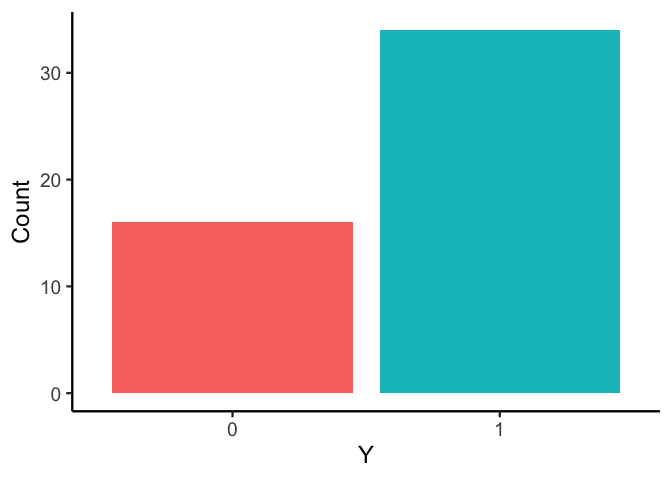
Now that we’ve said exactly how we’re collecting data and how much we’re collecting, it’s time to go ahead and collect that data. To demonstrate, let’s say you’ve got a coin and you want to know whether it’s a fair coin (that is, whether it lands equally on heads and tails). We’ll call the (unknown) probability that the coin lands on heads θ, and so we want to know if θ = 0.5. To test this, you can simply flip the coin N = 50 times and see what happens (here we use the rbinom function to randomly sample 0’s and 1’s, representing tails and heads, respectively):

1
2
3
4
5
coin_flip <- function(N, P) rbinom(N, 1, P)

THETA <- 0.7
N <- 50
Y <- coin_flip(N, THETA)

Step 3: Calculate a test statistic

The next thing we want is a summary of our data in the form of a statistic. Here, we just want to know whether θ = 0.5, so we calculate a t statistic with the mean under the null hypothesis equal to 0.5. Normally we’d use the t.test function to do this, but here I wrote out the formula so that we can calculate the p value manually.

1
2
3
t.value <- function (Y) (mean(Y) - 0.5) / (sd(Y) / sqrt(N))
t <- t.value(Y)
t

1
## [1] 2.701103

Step 4: Simulate some data, assuming H₀

That t statistic looks like something, but how do I know if it is significant? To determine significance, we need to find out what kind of t statistics we would get if the null hypothesis were true. Normally we do this using formulas, but what we’re really doing is simulating our experiment under the assumption of the null hypothesis. So let’s simulate 10000 experiments on a fair coin using replicate:

1
dt.h0 <- replicate(10000, t.value(coin_flip(N, 0.5)))

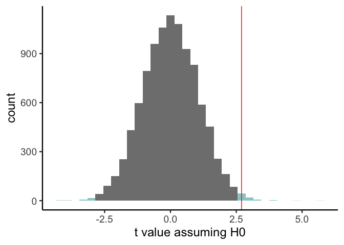
Step 5: How likely is this statistic under H₀?

We can see that our actual t statistic (the red line above) looks like it’s larger than most of the simulated values. To quantify exactly how much larger it is, we can simply count the proportion of simulated values that are at least as extreme as the value we got (the areas highlighted in blue above). This is our p value:

1
2
p <- mean(abs(dt.h0) >= abs(t))
writeLines(sprintf('t: %.2f\t\tp: %.2f', t, p))

1
## t: 2.70      p: 0.01

Wrapping it all up

We’ve seen that, perhaps counter to intuition, p values refer to the probability that you would have seen a statistic as extreme as the one you found if the null hypothesis were true. As much as we would like p values to tell us how probable the null hypothesis is given the data, they’re really just telling us how probable our results are given the null hypothesis.

You might think that wrapping your head around p values is the end of our troubles, but you’d be wrong. Let’s look at some other complications:

What if my testing intentions change?

Imagine you run an online study, and throw in some exploratory questions for kicks. You start to find that one of these exploratory questions, in addition to your question of interest, also exhibits an effect. Can you report both of these tests together?

Not without correction. Your p value assumes that you’re only performing one test, and doing two doubles your false positive rate (the probability that you reject H₀ even though it’s true). You can get around this by performing adjustments for multiple comparisons, but this can be hard to keep track of, so it’s not uncommon to see published articles with uncorrected (read: useless) p values.

What if my stopping intentions change?

Say you plan on collecting 50 EEG participants for a study. But, an unexpected pandemic happened, so you were only able to collect 40 participants before the world shut down. Can you run a t test with df = 39?

No. Since your testing intentions now involve availability (and not collecting until fixed N), your sample size is now a random variable. That is, it’s possible that you could have been able to squeeze in 38 or 45 participants instead of 40. This makes the Student t distribution unsuited for your analysis.

Does a small p value mean a large effect?

It’s fairly well known at this point that p values don’t indicate effect size or importance, but the temptation to treat p values as if they do carry this information persists.

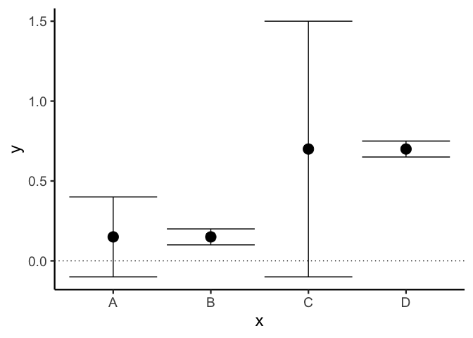
To see why they don’t, take a look at the following example. Despite the fact that both study A and study B show the same small effects, the p value for study A is non-significant while the p value for study B is significant. Likewise, even though study C and study D both show the same large effect, the effect is only significant for study D.

Is my parameter estimate probable?

Imagine that in an experiment you get the effect size shown above for study A. What’s the most likely size of the true effect over the population?

It could be anywhere. These confidence intervals tell you which effect sizes would be significantly different from the observed effect size, but they don’t tell you how probable any of these values are.

Is the null hypothesis ever true?

You get a “non-significant” p value of 0.4. Does this mean that the null hypothesis is true?

Nope. With traditional null hypothesis significance testing, you can never show support for the null hypothesis. You can only show evidence against it. Moreover, as we noted earlier, you can never know the probability of any hypothesis using Frequentist statistics.

Can Bayes do better?

Clearly, we’re running into some major issues with Frequentist statistics. Every time we want to know something, Frequentist statistics gives us something that masquerades as what we want, and we only find out that it was a sham after close inspection. Usually by then it’s too late. Mostly, the problem comes from one source: Frequentist statistics are based on possible outcomes under the null hypothesis constrained by one’s testing and stopping intentions. Since Frequentists define significance in this way, they need to be extremely careful in defining, adhering to, and interpreting results relative to testing and stopping intentions.

By contrast, Bayesian statisticians only care about one thing, and it’s disgusting: updating beliefs in light of observation. Bayesian statistics can be described most simply by its defining equation derived by, you guessed it, Thomas Bayes (the handsome Reverend at the top of this post). Here’s the equation:

Let’s break it down. The left hand size, P(θ|D), is the probability of our statistic given the data. We call this the posterior. Thankfully, we can tell right away that this is what we want, what Frequentist statistics wouldn’t give us. On the right hand side, we have two components.

The Prior

We call the first term, P(θ), our prior belief about θ (or just the prior). This says how likely we believe that any given value of θ is without any other information. There’s a lot of discussion as to how exactly to choose a prior, but there are a couple categories of priors that should help narrow it down.

• Improper/Flat Prior: I literally have no idea what θ looks like (e.g., P(θ) = Uniform(-∞, ∞))
• Vague Prior: θ is most likely to be 0, but I wouldn’t be surprised if it were absolutely massive either (e.g., P(θ) = N(0, 100000))
• Weakly Informative Prior: θ is probably somwhere between -25 and 25 (e.g., P(θ) = N(0, 10))
• Informative Prior: The last study on this topic said that θ is 27 (e.g., P(θ) = N(27, 1))

The Likelihood

The last part of this equation is P(D|θ), the likelihood of the data given θ. If this sounds familiar, it is: this is exactly what we were estimating in Frequentist statistics. You might have heard of “maximum likelihood estimation,” which is how a lot of Frequentist models are fitted.

The Posterior

Given a prior and a likelihood, we can compute our posterior just by multiplying the two together and normalizing so that the area of the distribution is equal to 1. In most cases this will be too inefficient, however, so usually we’ll resort to sampling algorithms to approximate the posterior instead of directly computing it.

Putting it all together

Let’s make this more concrete using the coin flipping example from above. The code below takes a range of values of θ, computes the likelihood of the data for each value of θ, and multiplies that likelihood by a uniform prior over the range [0, 1]:

1
2
3
4
5
6
7
8
9
10
11
12
normalize <- function(x) x / sum(x)
prior.beta <- function(theta, alpha=1, beta=1) dbeta(theta, alpha, beta)
L <- function(Y, theta) exp(sum(log(dbinom(Y, 1, theta))))

df <- expand_grid(theta=seq(0, 1, 0.01)) %>%
    group_by(theta) %>%
    summarize(likelihood=L(Y, theta),
              prior=prior.beta(theta)) %>%
    ungroup() %>%
    mutate(prior=normalize(prior),
           likelihood=normalize(likelihood),
           posterior=normalize(likelihood * prior))

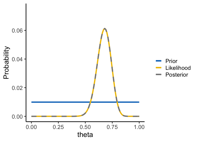
As you can see, when the prior is uniform, we get a posterior that exactly matches our data likelihood. Since Frequentist models often use the maximum likelihood parameter value, the mode of our posterior distribution tells us the Frequentist estimate. But since our posterior is a distribution, we know that the maximum likelihood estimate (the estimate that makes the data most likely) is also the most probable given the data. Likewise, any credible interval will tell us where the most probable values of θ all lie.

But the fun doesn’t stop there- you’re probably wondering how Bayesian statistics handles all of the problems we mentioned with Frequentist statistics. So let’s go through them one by one.

What if my testing intentions change?

Imagine you run an online study, and throw in some exploratory questions for kicks. You start to find that one of these exploratory questions, in addition to your question of interest, also exhibits an effect. Can you report both of these tests together?

Yup! Since Bayesian statistics depend on prior beliefs instead of testing and stopping intentions, you can run the additional analyses without worry.

What if my stopping intentions change?

Say you plan on collecting 50 EEG participants for a study. But, an unexpected pandemic happened, so you were only able to collect 40 participants before the world shut down. Can you run a Bayesian test on this data?

Yes! Again, since Bayesian statistics don’t rely on stopping intentions, you’re free to analyze this data. What’s perhaps even more impressive is that if you find that 40 participants isn’t enough data to differentiate between hypotheses, you can always go back, collect more data, and analyze the whole lot together in a Bayesian analysis (Rouder 2014). In Frequentist statistics this is called p hacking, and it can lead to all sorts of mistaken and worrying results.

Does a small p value mean a large effect?

Just like in Frequentist statistics, there are also different ways to quantify significance in Bayesian statistics. Bayes Factors are often used for hypothesis testing, since they tell you the odds of H₀ vs H_a. But a recent trend in Bayesian stats argues for focusing on parameter estimation, and not only hypothesis testing (Kruschke & Liddell, 2018). Ultimately, you still want to differentiate between how likely a hypothesis is, and how large the effect of interest is.

Is my parameter estimate probable?

Imagine that in an experiment you get the effect size shown above for study A. What’s the most likely size of the true effect over the population?

As we said before, in Bayesian statistics, the posterior mode is always the most probable value of a parameter! Likewise, the 95% credible interval tells you where the 95% most probable values of the parameter lie.

Is the null hypothesis ever true?

Using Bayes Factors, you can indeed confirm the null hypothesis! While it might not sound like the most interesting thing to confirm the null hypothesis, this is often an explicit goal of research. It’s also good to know the difference between “H₀ is probably true” and “the data can’t discriminate between H₀ and H_a.”

Bonus points

• Access to more types of distributions
• Access to more complex model structures (e.g., unequal variances)
• Easy calculation of CIs for multilevel models
• Easy model comparison & model averaging
• Planning for precision and power analyses
• Results are relatively insensitive to most choices of prior distributions
• When results are sensitive to priors, this may be an advantage if your priors are regularizing against overfitting

We’ve covered a lot of material in one blog, but I hope that I’ve made a case that Bayesian statistics are the answer to a lot of ongoing problems with Frequentist statistics. Look out for upcoming posts on the practical details of Bayesian analyses, which will cover the ins and outs of converting your workflow to be Bayesian!

References

Cassidy, S. A., Dimova, R., Giguère, B., Spence, J. R., & Stanley, D. J. (2019). Failing grade: 89% of introduction-to-psychology textbooks that define or explain statistical significance do so incorrectly. Advances in Methods and Practices in Psychological Science, 2(3), 233-239.

Kline, R. B. (2004). Beyond significance testing: Reforming data analysis methods in behavioral research.

Kruschke, J. K., & Liddell, T. M. (2018). The Bayesian New Statistics: Hypothesis testing, estimation, meta-analysis, and power analysis from a Bayesian perspective. Psychonomic Bulletin & Review, 25(1), 178-206.

Rouder, J. N. (2014). Optional stopping: No problem for Bayesians. Psychonomic bulletin & review, 21(2), 301-308.