
Intro to Bayesian Regression in R

Welcome! This is an intro-level workshop about Bayesian mixed effects
regression in R. We’ll cover the basics of Bayesian linear and logit
models. You should have an intermediate-level understanding of R and
Frequentist linear regression (using e.g. lm and lmer in R).
Acknowledgments: To make our analyses directly comparable to analyses we’ve already covered, this workshop is directly copied from Allie’s awesome workshop on Frequentist mixed-effect regression. That workshop was adapted from code provided by Gabriela K Hajduk, who in turn referenced a workshop developed by Liam Bailey. Parts of the tutorial are also adapted from a lesson on partial pooling by Tristan Mahr.
For further reading, please check out their tutorials and blogs here:
https://gkhajduk.github.io/2017-03-09-mixed-models/
https://www.tjmahr.com/plotting-partial-pooling-in-mixed-effects-models/
Setup
First, we’ll just get everything set up. We need to tweak some
settings, load packages, and read our data.
1
2
3
4
5
6
7
8
9
10
11
12
13
14
15
16
17
18
19
20
21
22
#change some settings
options(contrasts = c("contr.sum","contr.poly"))
#this tweaks makes sure that contrasts are interpretable as main effects

#time to load some packages!
library(lme4) #fit the models
library(lmerTest) #gives p-values and more info
library(car) #more settings for regression output
library(tidyr) #for data wrangling
library(dplyr) #for data wrangling
library(tibble) #for data wrangling
library(ggplot2) #plotting raw data
library(data.table) #for pretty HTML tables of model parameters

library(brms)       # bayesian regression!
library(emmeans)    # used to get predicted means per condition
library(modelr)     # used to get predicted means per condition
library(tidybayes)  # for accessing model posteriors
library(bayestestR) # for testing over posteriors

#load the data
dragons <- read.csv("2020-10-21-dragon-data.csv")
Data
Let’s get familiar with our dataset. This is a fictional dataset about dragons. Each dragon has one row. We have information about each dragon’s body length and cognitive test score. Let’s say our first research question is whether the length of the dragon is related to its intelligence.
We also have some other information about each dragon: We know about the mountain range where it lives, its color, its diet, and whether or not it breathes fire.
Let’s take a look at the data and check the counts of our variables:
1
2
3
4
5
6
7
8
# take a peek at the header
head(dragons)

#check out counts for all our categorical variables
table(dragons$mountainRange)
table(dragons$diet)
table(dragons$color)
table(dragons$breathesFire)
1
2
3
4
5
6
7
8
9
10
11
12
13
14
15
16
17
18
19
##    testScore bodyLength mountainRange color      diet breathesFire
## 1  0.0000000   175.5122      Bavarian  Blue Carnivore            1
## 2  0.7429138   190.6410      Bavarian  Blue Carnivore            1
## 3  2.5018247   169.7088      Bavarian  Blue Carnivore            1
## 4  3.3804301   188.8472      Bavarian  Blue Carnivore            1
## 5  4.5820954   174.2217      Bavarian  Blue Carnivore            0
## 6 12.4536350   183.0819      Bavarian  Blue Carnivore            1
##
## Bavarian  Central Emmental   Julian Ligurian Maritime  Sarntal Southern
##       60       60       60       60       60       60       60       60
##
##  Carnivore   Omnivore Vegetarian
##        156        167        157
##
##   Blue    Red Yellow
##    160    160    160
##
##   0   1
## 229 251
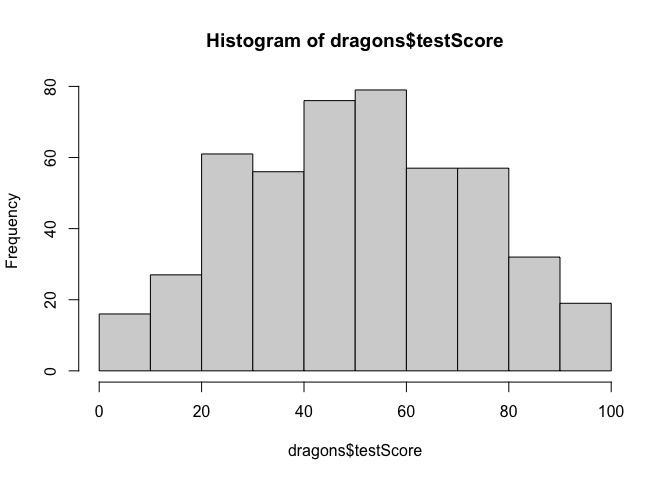
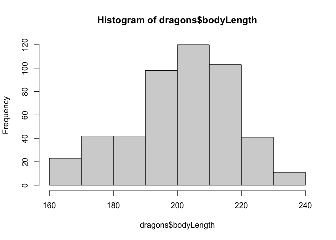
Now let’s check distributions. Do test scores and body length measurements look approximately normal?
1
2
#check assumptions: do our continuous variables have approximately normal distributions?
hist(dragons$testScore)
1
hist(dragons$bodyLength)
Bayesian Linear Regression
Okay, let’s start fitting some lines! Key Question: Does body
length predict test score?
One way to analyse this data would be to try fitting a linear model to all our data, ignoring all the other variables for now. To make sure that we can interpret our coefficients, we should mean-center our continuous measure of body length before using it in a model.
This is a “complete pooling” approach, where we “pool” together all the data and ignore the fact that some observations came from specific mountain ranges.
1
2
model <- lm(testScore ~ scale(bodyLength), data = dragons)
summary(model)
1
2
3
4
5
6
7
8
9
10
11
12
13
14
15
16
17
18
##
## Call:
## lm(formula = testScore ~ scale(bodyLength), data = dragons)
##
## Residuals:
##     Min      1Q  Median      3Q     Max
## -56.962 -16.411  -0.783  15.193  55.200
##
## Coefficients:
##                   Estimate Std. Error t value Pr(>|t|)
## (Intercept)        50.3860     0.9676  52.072   <2e-16 ***
## scale(bodyLength)   8.9956     0.9686   9.287   <2e-16 ***
## ---
## Signif. codes:  0 '***' 0.001 '**' 0.01 '*' 0.05 '.' 0.1 ' ' 1
##
## Residual standard error: 21.2 on 478 degrees of freedom
## Multiple R-squared:  0.1529, Adjusted R-squared:  0.1511
## F-statistic: 86.25 on 1 and 478 DF,  p-value: < 2.2e-16
Incredible! It’s super significant! We’re gonna publish in Nature
Dragonology! How can we run an analogous Bayesian regression to get full
posterior distributions of our coefficient? Since we standardized body
length, it might be reasonable to set a normal(0, sd(testScore)) prior
over the effect of body length, which says that we expect a unit
increase in body length to yield on the order of somewhere between a
unit decrease and a unit increase in test score. The code is mostly the
same except that we use the brm function instead of lm, we specify a
file to store our model in (so we don’t have to fit it multiple times),
and we specify our normal prior for the model coefficients:
1
2
3
model.bayes <- brm(testScore ~ scale(bodyLength),
                   data=dragons, file='bodyLength',
                   prior=set_prior(paste0('normal(0, ', sd(dragons$testScore), ')')))
1
2
3
4
5
6
7
8
9
10
11
12
13
14
15
16
17
18
19
20
21
22
23
24
25
26
27
28
29
30
31
32
33
34
35
36
37
38
39
40
41
42
43
44
45
46
47
48
49
50
51
52
53
54
55
56
57
58
59
60
61
62
63
64
65
66
67
68
69
70
71
72
73
74
75
76
77
78
79
80
81
82
83
84
85
86
87
88
89
90
91
92
93
94
95
96
97
98
99
100
##
## SAMPLING FOR MODEL '49f78aecf53dc588372d55583a8e39cb' NOW (CHAIN 1).
## Chain 1:
## Chain 1: Gradient evaluation took 2.6e-05 seconds
## Chain 1: 1000 transitions using 10 leapfrog steps per transition would take 0.26 seconds.
## Chain 1: Adjust your expectations accordingly!
## Chain 1:
## Chain 1:
## Chain 1: Iteration:    1 / 2000 [  0%]  (Warmup)
## Chain 1: Iteration:  200 / 2000 [ 10%]  (Warmup)
## Chain 1: Iteration:  400 / 2000 [ 20%]  (Warmup)
## Chain 1: Iteration:  600 / 2000 [ 30%]  (Warmup)
## Chain 1: Iteration:  800 / 2000 [ 40%]  (Warmup)
## Chain 1: Iteration: 1000 / 2000 [ 50%]  (Warmup)
## Chain 1: Iteration: 1001 / 2000 [ 50%]  (Sampling)
## Chain 1: Iteration: 1200 / 2000 [ 60%]  (Sampling)
## Chain 1: Iteration: 1400 / 2000 [ 70%]  (Sampling)
## Chain 1: Iteration: 1600 / 2000 [ 80%]  (Sampling)
## Chain 1: Iteration: 1800 / 2000 [ 90%]  (Sampling)
## Chain 1: Iteration: 2000 / 2000 [100%]  (Sampling)
## Chain 1:
## Chain 1:  Elapsed Time: 0.052493 seconds (Warm-up)
## Chain 1:                0.043537 seconds (Sampling)
## Chain 1:                0.09603 seconds (Total)
## Chain 1:
##
## SAMPLING FOR MODEL '49f78aecf53dc588372d55583a8e39cb' NOW (CHAIN 2).
## Chain 2:
## Chain 2: Gradient evaluation took 1.3e-05 seconds
## Chain 2: 1000 transitions using 10 leapfrog steps per transition would take 0.13 seconds.
## Chain 2: Adjust your expectations accordingly!
## Chain 2:
## Chain 2:
## Chain 2: Iteration:    1 / 2000 [  0%]  (Warmup)
## Chain 2: Iteration:  200 / 2000 [ 10%]  (Warmup)
## Chain 2: Iteration:  400 / 2000 [ 20%]  (Warmup)
## Chain 2: Iteration:  600 / 2000 [ 30%]  (Warmup)
## Chain 2: Iteration:  800 / 2000 [ 40%]  (Warmup)
## Chain 2: Iteration: 1000 / 2000 [ 50%]  (Warmup)
## Chain 2: Iteration: 1001 / 2000 [ 50%]  (Sampling)
## Chain 2: Iteration: 1200 / 2000 [ 60%]  (Sampling)
## Chain 2: Iteration: 1400 / 2000 [ 70%]  (Sampling)
## Chain 2: Iteration: 1600 / 2000 [ 80%]  (Sampling)
## Chain 2: Iteration: 1800 / 2000 [ 90%]  (Sampling)
## Chain 2: Iteration: 2000 / 2000 [100%]  (Sampling)
## Chain 2:
## Chain 2:  Elapsed Time: 0.064402 seconds (Warm-up)
## Chain 2:                0.035814 seconds (Sampling)
## Chain 2:                0.100216 seconds (Total)
## Chain 2:
##
## SAMPLING FOR MODEL '49f78aecf53dc588372d55583a8e39cb' NOW (CHAIN 3).
## Chain 3:
## Chain 3: Gradient evaluation took 1.2e-05 seconds
## Chain 3: 1000 transitions using 10 leapfrog steps per transition would take 0.12 seconds.
## Chain 3: Adjust your expectations accordingly!
## Chain 3:
## Chain 3:
## Chain 3: Iteration:    1 / 2000 [  0%]  (Warmup)
## Chain 3: Iteration:  200 / 2000 [ 10%]  (Warmup)
## Chain 3: Iteration:  400 / 2000 [ 20%]  (Warmup)
## Chain 3: Iteration:  600 / 2000 [ 30%]  (Warmup)
## Chain 3: Iteration:  800 / 2000 [ 40%]  (Warmup)
## Chain 3: Iteration: 1000 / 2000 [ 50%]  (Warmup)
## Chain 3: Iteration: 1001 / 2000 [ 50%]  (Sampling)
## Chain 3: Iteration: 1200 / 2000 [ 60%]  (Sampling)
## Chain 3: Iteration: 1400 / 2000 [ 70%]  (Sampling)
## Chain 3: Iteration: 1600 / 2000 [ 80%]  (Sampling)
## Chain 3: Iteration: 1800 / 2000 [ 90%]  (Sampling)
## Chain 3: Iteration: 2000 / 2000 [100%]  (Sampling)
## Chain 3:
## Chain 3:  Elapsed Time: 0.058688 seconds (Warm-up)
## Chain 3:                0.038065 seconds (Sampling)
## Chain 3:                0.096753 seconds (Total)
## Chain 3:
##
## SAMPLING FOR MODEL '49f78aecf53dc588372d55583a8e39cb' NOW (CHAIN 4).
## Chain 4:
## Chain 4: Gradient evaluation took 1.3e-05 seconds
## Chain 4: 1000 transitions using 10 leapfrog steps per transition would take 0.13 seconds.
## Chain 4: Adjust your expectations accordingly!
## Chain 4:
## Chain 4:
## Chain 4: Iteration:    1 / 2000 [  0%]  (Warmup)
## Chain 4: Iteration:  200 / 2000 [ 10%]  (Warmup)
## Chain 4: Iteration:  400 / 2000 [ 20%]  (Warmup)
## Chain 4: Iteration:  600 / 2000 [ 30%]  (Warmup)
## Chain 4: Iteration:  800 / 2000 [ 40%]  (Warmup)
## Chain 4: Iteration: 1000 / 2000 [ 50%]  (Warmup)
## Chain 4: Iteration: 1001 / 2000 [ 50%]  (Sampling)
## Chain 4: Iteration: 1200 / 2000 [ 60%]  (Sampling)
## Chain 4: Iteration: 1400 / 2000 [ 70%]  (Sampling)
## Chain 4: Iteration: 1600 / 2000 [ 80%]  (Sampling)
## Chain 4: Iteration: 1800 / 2000 [ 90%]  (Sampling)
## Chain 4: Iteration: 2000 / 2000 [100%]  (Sampling)
## Chain 4:
## Chain 4:  Elapsed Time: 0.052508 seconds (Warm-up)
## Chain 4:                0.041537 seconds (Sampling)
## Chain 4:                0.094045 seconds (Total)
## Chain 4:
1
summary(model.bayes, prior=TRUE)
1
2
3
4
5
6
7
8
9
10
11
12
13
14
15
16
17
18
19
20
21
22
23
24
##  Family: gaussian
##   Links: mu = identity; sigma = identity
## Formula: testScore ~ scale(bodyLength)
##    Data: dragons (Number of observations: 480)
## Samples: 4 chains, each with iter = 2000; warmup = 1000; thin = 1;
##          total post-warmup samples = 4000
##
## Priors:
## b ~ normal(0, 23.0088071104418)
## Intercept ~ student_t(3, 51, 26.1)
## sigma ~ student_t(3, 0, 26.1)
##
## Population-Level Effects:
##                 Estimate Est.Error l-95% CI u-95% CI Rhat Bulk_ESS Tail_ESS
## Intercept          50.37      0.98    48.46    52.22 1.00     3608     2184
## scalebodyLength     8.98      0.95     7.14    10.86 1.00     3939     3218
##
## Family Specific Parameters:
##       Estimate Est.Error l-95% CI u-95% CI Rhat Bulk_ESS Tail_ESS
## sigma    21.25      0.67    19.96    22.59 1.00     3826     3030
##
## Samples were drawn using sampling(NUTS). For each parameter, Bulk_ESS
## and Tail_ESS are effective sample size measures, and Rhat is the potential
## scale reduction factor on split chains (at convergence, Rhat = 1).
After waiting a minute for the model to compile and fit, we can see that
this summary gives us a little more information than lm did. First, it
tells us some basics about our model: the noise distribution family is
Gaussian with an identity link function, and so on. Next it tells us
what our priors are. In this case, brms uses default Student t priors
for the intercept and for the standard deviation, and our specified
normal prior for the regression slope. Finally, brms tells us about
our results. Here Estimate is the posterior mean (which is the most
likely for unimodal/symmetric distributions), Est.Error is the
standard deviation of the posterior (kind of like the standard error),
and l-95% CI and u-95% CI are the credible intervals (values inside
this range are the 95% most probable values). We also get some
convergence information for each parameter (Rhat, Bulk_ESS, and
Tail_ESS), which we’ll talk about later.
You also might be wondering what the heck is the deal with all those
chain outputs. Those are just updates on the algorithm brms uses to
compute the posterior. It’s called Markov-Chain Monte Carlo (MCMC)
sampling and you can learn more about it
here
if you’re interested.
To perform significance testing on our Bayesian regression model, we can
use the nifty describe_posterior function from the bayestestR
package, which computes a bunch of different tests for us:
1
2
describe_posterior(model.bayes, ci=.95, rope_ci=.95,
                   test=c('pd', 'p_map', 'rope', 'bf'))
1
2
3
4
5
6
## # Description of Posterior Distributions
##
## Parameter       | Median |           95% CI | p_MAP |      pd |        95% ROPE | % in ROPE |        BF |  Rhat |      ESS
## --------------------------------------------------------------------------------------------------------------------------
## Intercept       | 50.384 | [48.511, 52.268] |     0 | 100.00% | [-2.301, 2.301] |         0 | 6.641e+52 | 1.000 | 3539.342
## scalebodyLength |  8.971 | [ 7.218, 10.889] |     0 | 100.00% | [-2.301, 2.301] |         0 | 1.316e+06 | 1.000 | 3922.522
Like before, this gives us summaries of our posterior (in this case the
median and 95% CI). But this time we also see two measures of effect
existence, analogous to p-values on Frequentist approaches. p_MAP is
the posterior density at 0 divided by the posterior density at the mode,
and is on the same scale as a p-value. pd is the probability of
direction, which is the percentage of the posterior that all has the
same sign (whichever is greater). We also get two measures of effect
significance: the % in ROPE tells us how much of the posterior is
inside a null region (in this case a standardized effect size of <
.1), and BF is a Bayes Factor, where BF > 1 indicates support for
the alternative hypothesis and BF < 1 indicates support for the null
hypothesis. There is a whole lot of discussion about which of these
metrics are best to use, and we could take a whole meeting talking about
this. But for now, we can take solace that all of the measures agree-
just like we saw before, it looks like the effect of body length is
significant!
We saw that the estimates and inferences from both models look similar,
but let’s plot the data with ggplot2 to see how much they actually
overlap.
1
2
3
4
5
6
7
8
9
10
11
12
13
14
15
16
17
18
19
lm.emm <- emmeans(model, ~bodyLength,
                  at=list(bodyLength=seq(min(dragons$bodyLength),
                                         max(dragons$bodyLength)))) %>%
    as.data.frame
brm.emm <- emmeans(model.bayes, ~bodyLength,
                   at=list(bodyLength=seq(min(dragons$bodyLength),
                                          max(dragons$bodyLength)))) %>%
    as.data.frame

ggplot(dragons, aes(x=bodyLength, y=testScore)) +
    geom_point() +
    geom_line(aes(y=emmean, color='lm'), data=lm.emm) +
    geom_ribbon(aes(y=emmean, ymin=lower.CL, ymax=upper.CL, fill='lm'),
                data=lm.emm, alpha=0.4) +
    geom_line(aes(y=emmean, color='brm'), data=brm.emm) +
    geom_ribbon(aes(y=emmean, ymin=lower.HPD, ymax=upper.HPD, fill='brm'),
                data=brm.emm, alpha=0.4) +
    xlab("Body Length") +
    ylab("Test Score") + theme_minimal()
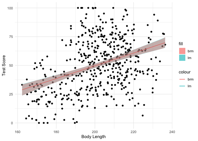
As you can see, the fitted lines and 95% CIs look almost exactly the same between the two different approaches. Then why bother waiting for a Bayesian model to fit? Because instead of just an estimate and a confidence interval, we get a full posterior distribution over our model coefficients that allows us to directly infer the most probable values:
1
plot(model.bayes)
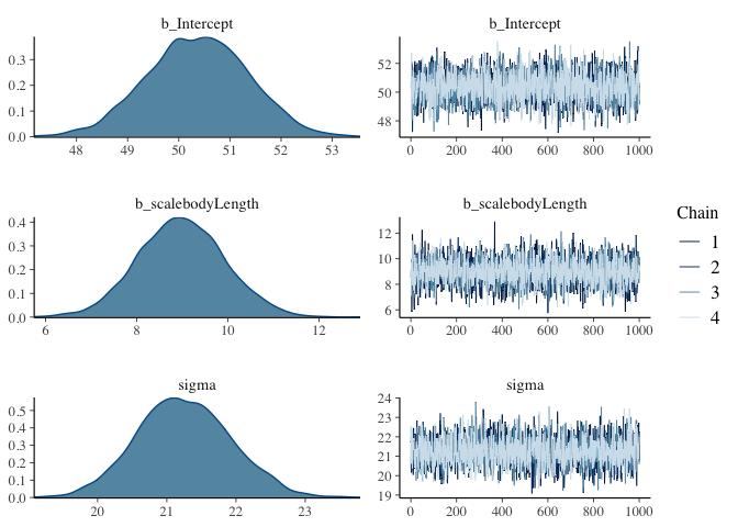
From these plots, we can see that the average test score is most likely about 50, but could also be somewhere between 48 and 53. Similarly, we can see that a unit increase in body length is most likely to yield an increase in 9 points of test score, and that the standard deviation in test scores is probably around 21 test points. With our Frequentist regression, we can predict that these values make the observed data most likely, but we can’t directly make inferences about how probable the values are.
Then what are the squiggly things on the right side? Since most
regression models don’t have easy analytic solutions, we have to sample
from our posterior distribution instead of calculating it directly. The
lines are called MCMC chains, the x-axis is the number of each sample
and the y-axis is the value of each sample. For now, all you need to
know is that if the chains look like nice fuzzy caterpillars (like they
do here), then our model has converged. Otherwise, brms will give us
some warnings that things went awry, and will give us advice for how to
solve the problem.
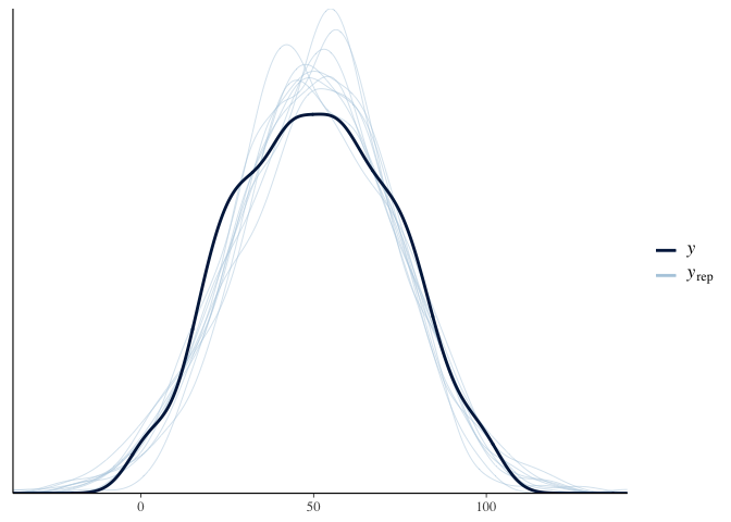
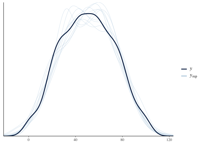
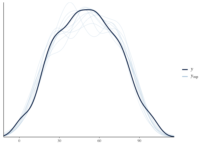
Another benefit of brms is that we can use it to simulate test scores
and see how well it covers the actual distribution of test scores. This
is called a “posterior predictive check.” Here the dark line is the
actual distribution of test scores, and each light line is the
distribution of test scores predicted by a single sample of the
posterior. Since the light lines mostly cover the solid line, it looks
like our model fits the data fairly well:
1
pp_check(model.bayes)
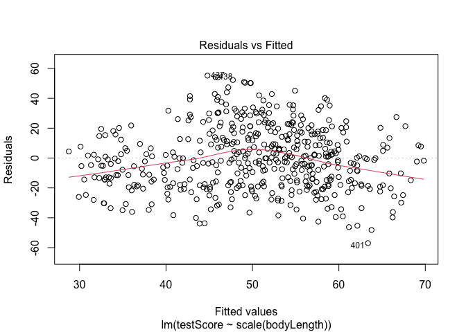
But before we make any grand conclusions, we need to check that we met
assumptions! We can use plot for the Frequentist lm model. To check
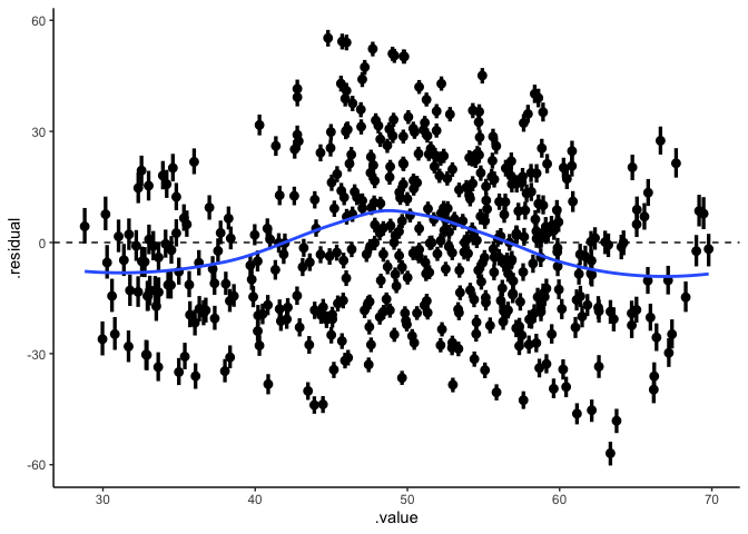
the assumptions of the Bayesian model, we can use add_residual_draws
from the tidybayes package to get the residual posterior for each data
point.
1
2
3
4
5
6
7
draws <- full_join(add_fitted_draws(dragons, model.bayes),
                   add_residual_draws(dragons, model.bayes)) %>%
    group_by(.row) %>%
    median_hdi(.value, .residual)

## Let's plot the residuals from this model. Ideally, the red line should be flat.
plot(model, which = 1)  # not perfect, but looks alright
1
2
3
4
5
6
ggplot(draws, aes(x=.value, xmin=.value.lower, xmax=.value.upper,
                  y=.residual, ymin=.residual.lower, ymax=.residual.upper)) +
    geom_pointinterval() +
    geom_hline(yintercept=0, linetype='dashed') +
    stat_smooth(se=FALSE) +
    theme_classic()
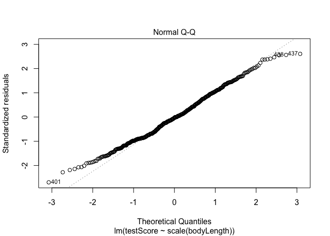
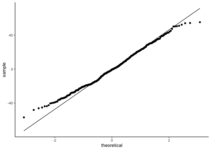
1
2
## Have a quick look at the  qqplot too - point should ideally fall onto the diagonal dashed line
plot(model, which = 2)  # a bit off at the extremes, but that's often the case; again doesn't look too bad
1
2
3
4
ggplot(draws, aes(sample=.residual)) +
    geom_qq() +
    geom_qq_line() +
    theme_classic()
But linear models also assume that observations are INDEPENDENT. Uh oh.
We collected multiple samples from eight mountain ranges. It’s perfectly plausible that the data from within each mountain range are more similar to each other than the data from different mountain ranges - they are correlated. This could be a problem.
1
2
3
4
5
6
#Lets have a quick look at the data split by mountain range
#We use the facet_wrap to do that
ggplot(data = dragons, aes(x = bodyLength, y = testScore)) +
  geom_point() +
  facet_wrap(.~mountainRange) +
  xlab("length") + ylab("test score")
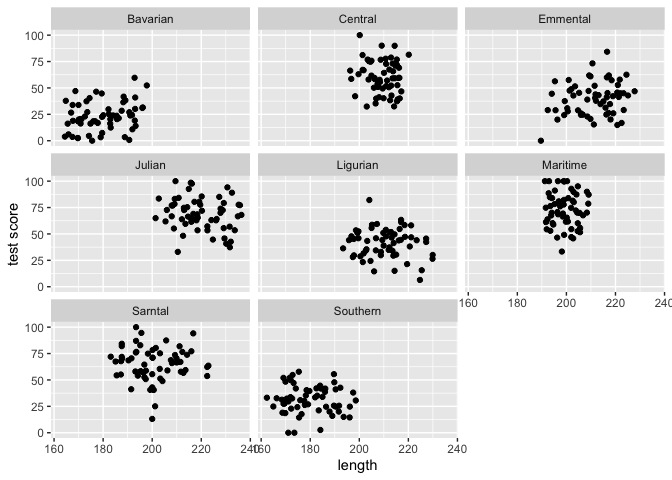
From the above plots it indeed looks like our mountain ranges vary both in the dragon body length and in their test scores. This confirms that our observations from within each of the ranges aren’t independent. We can’t ignore that.
Bayesian Multilevel Linear Regression
Mountain range clearly introduces a structured source of variance
in our data. We need to control for that variation if we want to
understand whether body length really predicts test scores.
Multilevel regression is a compromise: Partial pooling! We can let each mountain range have its own regression line, but make an informed guess about that line based on the group-level estimates. This is especially useful when some groups/participants have incomplete data.
Note that here we use the term “multilevel” or “hierarchical” instead of “mixed effect” regression. This is because in a Bayesian framework, all of your effects are modeled as “random” effects! In Frequentist regression, “random” effects are just normal effects that are modeled with an underlying standard normal distribution: in other words, they’re modeled with a standard normal prior. Since all effects in Bayesian regressions have priors, it’s easier and more precise to refer to population-level effects (akin to “fixed” effects) and group-level effects (akin to “random” effects).
Should Mountain Range be a Population-level or Group-level effect?
Since we want to estimate the mean effect of body-length over all mountain ranges, we want a population-level effect of body length. But since we also think that mountain ranges could have different mean test scores and different effects of body length, we also want separate group-level effects over mountain ranges.
Here’s how we did this with lmer:
1
2
3
4
5
#let's fit our first multilevel model!
multilevel_model <- lmer(testScore ~ scale(bodyLength) + (1+scale(bodyLength)|mountainRange), data = dragons)

#what's the verdict?
summary(multilevel_model)
1
2
3
4
5
6
7
8
9
10
11
12
13
14
15
16
17
18
19
20
21
22
23
24
25
26
27
28
29
30
31
## Linear mixed model fit by REML. t-tests use Satterthwaite's method [
## lmerModLmerTest]
## Formula:
## testScore ~ scale(bodyLength) + (1 + scale(bodyLength) | mountainRange)
##    Data: dragons
##
## REML criterion at convergence: 3980.5
##
## Scaled residuals:
##     Min      1Q  Median      3Q     Max
## -3.5004 -0.6683  0.0207  0.6592  2.9449
##
## Random effects:
##  Groups        Name              Variance Std.Dev. Corr
##  mountainRange (Intercept)       324.102  18.003
##                scale(bodyLength)   9.905   3.147   -1.00
##  Residual                        221.578  14.885
## Number of obs: 480, groups:  mountainRange, 8
##
## Fixed effects:
##                   Estimate Std. Error       df t value Pr(>|t|)
## (Intercept)       51.75302    6.40349  6.91037   8.082 9.16e-05 ***
## scale(bodyLength) -0.03326    1.68317 10.22337  -0.020    0.985
## ---
## Signif. codes:  0 '***' 0.001 '**' 0.01 '*' 0.05 '.' 0.1 ' ' 1
##
## Correlation of Fixed Effects:
##             (Intr)
## scl(bdyLng) -0.674
## optimizer (nloptwrap) convergence code: 0 (OK)
## boundary (singular) fit: see ?isSingular
Again, the Bayesian version with brms is essentially the same to run:
1
2
3
4
5
6
#let's fit our first mixed model!
multilevel_model.bayes <- brm(testScore ~ scale(bodyLength) + (1+scale(bodyLength)|mountainRange),
                              data=dragons, file='bodyLength_multilevel',
                              prior=set_prior(paste0('normal(0, ', sd(dragons$testScore), ')')))

summary(multilevel_model.bayes, prior=TRUE)
1
2
3
4
5
6
7
8
9
10
11
12
13
14
15
16
17
18
19
20
21
22
23
24
25
26
27
28
29
30
31
32
33
34
35
36
37
##  Family: gaussian
##   Links: mu = identity; sigma = identity
## Formula: testScore ~ scale(bodyLength) + (1 + scale(bodyLength) | mountainRange)
##    Data: dragons (Number of observations: 480)
## Samples: 4 chains, each with iter = 2000; warmup = 1000; thin = 1;
##          total post-warmup samples = 4000
##
## Priors:
## b ~ normal(0, 23.0088071104418)
## Intercept ~ student_t(3, 51, 26.1)
## L ~ lkj_corr_cholesky(1)
## sd ~ student_t(3, 0, 26.1)
## sigma ~ student_t(3, 0, 26.1)
##
## Group-Level Effects:
## ~mountainRange (Number of levels: 8)
##                                Estimate Est.Error l-95% CI u-95% CI Rhat
## sd(Intercept)                     20.63      5.92    12.19    35.13 1.00
## sd(scalebodyLength)                3.76      2.17     0.35     8.89 1.00
## cor(Intercept,scalebodyLength)    -0.55      0.39    -0.98     0.45 1.00
##                                Bulk_ESS Tail_ESS
## sd(Intercept)                      1362     1915
## sd(scalebodyLength)                1820     1699
## cor(Intercept,scalebodyLength)     3176     2620
##
## Population-Level Effects:
##                 Estimate Est.Error l-95% CI u-95% CI Rhat Bulk_ESS Tail_ESS
## Intercept          51.25      7.11    36.62    64.88 1.00     1040     1590
## scalebodyLength     0.12      1.97    -3.97     3.91 1.00     2340     1936
##
## Family Specific Parameters:
##       Estimate Est.Error l-95% CI u-95% CI Rhat Bulk_ESS Tail_ESS
## sigma    14.93      0.49    14.03    15.93 1.00     4904     2967
##
## Samples were drawn using sampling(NUTS). For each parameter, Bulk_ESS
## and Tail_ESS are effective sample size measures, and Rhat is the potential
## scale reduction factor on split chains (at convergence, Rhat = 1).
1
2
describe_posterior(multilevel_model.bayes, ci=.95, rope_ci=.95,
                   test=c('pd', 'p_map', 'rope', 'bf'))
1
2
3
4
5
6
## # Description of Posterior Distributions
##
## Parameter       | Median |           95% CI | p_MAP |      pd |        95% ROPE | % in ROPE |        BF |  Rhat |      ESS
## --------------------------------------------------------------------------------------------------------------------------
## Intercept       | 51.279 | [36.597, 64.809] | 0.000 | 100.00% | [-2.301, 2.301] |     0.000 | 91530.079 | 1.000 | 1018.165
## scalebodyLength |  0.200 | [-3.993,  3.871] | 0.979 |  54.57% | [-2.301, 2.301] |    82.163 |     0.078 | 1.000 | 2210.472
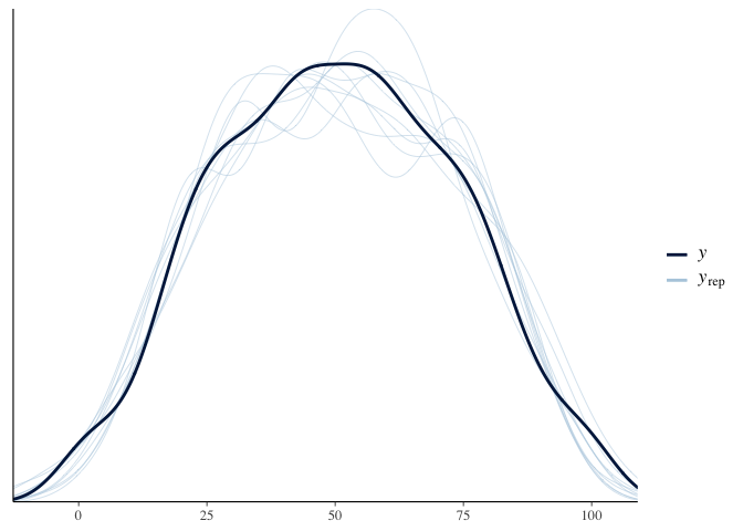
1
pp_check(multilevel_model.bayes)
The summary output for brms is pretty much the same as before,
except now we also have a section for group-level effects in addition to
our earlier section for Population-level effects. Since we estimated
separate intercepts and effects of body length on test score for each
mountain range, our model tells us the standard deviation of each of
those two effects, and also the correlation between them. The standard
deviations look fairly similar to the lmer values, but the correlation
looks much more reasonable than the lmer value (i.e., it’s no longer a
perfect negative correlation).
Overall, it looks like when we account for the effect of mountain range, there is no relationship between body length and test scores. This is true for both the Frequentist and the Bayesian regressions. Well, so much for our Nature Dragonology paper!
Unless… What about our other variables? Let’s test whether diet is related to test scores instead.
1
2
3
4
5
model.diet <- brm(testScore ~ diet + (1+diet|mountainRange),
                        data=dragons, file='diet_multilevel',
                        prior=set_prior(paste0('normal(0, ', sd(dragons$testScore), ')')))

summary(model.diet, prior=TRUE)
1
2
3
4
5
6
7
8
9
10
11
12
13
14
15
16
17
18
19
20
21
22
23
24
25
26
27
28
29
30
31
32
33
34
35
36
37
38
39
40
41
42
43
44
##  Family: gaussian
##   Links: mu = identity; sigma = identity
## Formula: testScore ~ diet + (1 + diet | mountainRange)
##    Data: dragons (Number of observations: 480)
## Samples: 4 chains, each with iter = 2000; warmup = 1000; thin = 1;
##          total post-warmup samples = 4000
##
## Priors:
## b ~ normal(0, 23.0088071104418)
## Intercept ~ student_t(3, 51, 26.1)
## L ~ lkj_corr_cholesky(1)
## sd ~ student_t(3, 0, 26.1)
## sigma ~ student_t(3, 0, 26.1)
##
## Group-Level Effects:
## ~mountainRange (Number of levels: 8)
##                      Estimate Est.Error l-95% CI u-95% CI Rhat Bulk_ESS
## sd(Intercept)           11.47      3.82     6.57    20.22 1.00     1311
## sd(diet1)                2.70      1.98     0.14     7.47 1.00      935
## sd(diet2)                4.92      2.01     1.85     9.86 1.00     1475
## cor(Intercept,diet1)     0.08      0.44    -0.79     0.83 1.00     3302
## cor(Intercept,diet2)     0.72      0.24     0.10     0.98 1.00     1950
## cor(diet1,diet2)        -0.29      0.43    -0.90     0.69 1.00     2261
##                      Tail_ESS
## sd(Intercept)            1923
## sd(diet1)                1867
## sd(diet2)                1961
## cor(Intercept,diet1)     2301
## cor(Intercept,diet2)     2866
## cor(diet1,diet2)         2887
##
## Population-Level Effects:
##           Estimate Est.Error l-95% CI u-95% CI Rhat Bulk_ESS Tail_ESS
## Intercept    49.45      4.16    41.08    57.96 1.00     1168     1650
## diet1       -15.02      1.61   -18.09   -11.41 1.00     2308     1715
## diet2        15.00      2.13    10.57    18.89 1.00     1653     1758
##
## Family Specific Parameters:
##       Estimate Est.Error l-95% CI u-95% CI Rhat Bulk_ESS Tail_ESS
## sigma    10.74      0.35    10.05    11.46 1.00     4776     2879
##
## Samples were drawn using sampling(NUTS). For each parameter, Bulk_ESS
## and Tail_ESS are effective sample size measures, and Rhat is the potential
## scale reduction factor on split chains (at convergence, Rhat = 1).
1
2
describe_posterior(model.diet, ci=.95, rope_ci=.95,
                   test=c('pd', 'p_map', 'rope', 'bf'))
1
2
3
4
5
6
7
## # Description of Posterior Distributions
##
## Parameter |  Median |             95% CI | p_MAP |      pd |        95% ROPE | % in ROPE |        BF |  Rhat |      ESS
## -----------------------------------------------------------------------------------------------------------------------
## Intercept |  49.455 | [ 40.919,  57.793] |     0 | 100.00% | [-2.301, 2.301] |         0 | 9.108e+08 | 1.001 | 1161.725
## diet1     | -15.090 | [-18.170, -11.587] |     0 | 100.00% | [-2.301, 2.301] |         0 |  2381.239 | 1.001 | 2050.769
## diet2     |  15.072 | [ 10.533,  18.810] |     0 | 100.00% | [-2.301, 2.301] |         0 |  2135.790 | 1.001 | 1639.868
1
pp_check(model.diet)
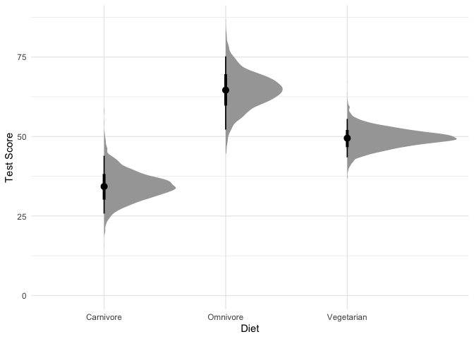
Visualizing the effect of diet on test scores predicted by our model will help us better understand what we just found:
1
2
3
4
5
6
7
8
#Plot average test score by diet type
dragons %>%
    data_grid(diet) %>%
    add_fitted_draws(model.diet, re_formula=NA) %>%
    ggplot(aes(x=diet, y=.value)) +
    stat_halfeye(point_interval=median_hdi) + ylim(0, NA) +
    xlab("Diet") + ylab("Test Score") +
    theme_minimal()
1
2
3
4
5
6
7
8
9
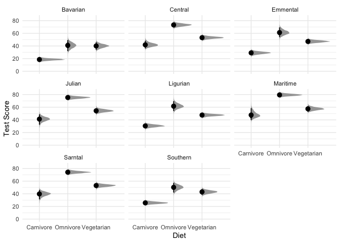
#Let's also look at the effect across mountain ranges.
dragons %>%
data_grid(diet, mountainRange) %>%
add_fitted_draws(model.diet) %>%
ggplot(aes(x=diet, y=.value)) +
stat_halfeye(point_interval=median_hdi) + ylim(0, NA) +
facet_wrap( ~ mountainRange) +
xlab("Diet") + ylab("Test Score") +
theme_minimal()
What are we looking at here? The black points represent the mode of the posterior, the thick black lines represent the 66% credible intervals, and the thinner black lines represnt the 95% credible intervals (also called highest density intervals). The curves in gray represent the full posterior distribution. A nice thing about using a Bayesian model is that instead of being stuck with ugly & often misleading bar charts, we can directly plot how likely each mean is along with the full posterior distribution.
In sum, these results look pretty consistent, but there’s clearly still variability among different mountains.
So far, so good. But what if we’re interested in testing multiple variables at the same time? We build a model with an interaction term!
1
2
3
4
5
model.diet.length <- brm(testScore ~ diet*scale(bodyLength) + (1 + diet*scale(bodyLength)|mountainRange),
                         data=dragons, file='diet_length',
                         prior=set_prior(paste0('normal(0, ', sd(dragons$testScore), ')')))

summary(model.diet.length, prior=TRUE)
1
2
3
4
5
6
7
8
9
10
11
12
13
14
15
16
17
18
19
20
21
22
23
24
25
26
27
28
29
30
31
32
33
34
35
36
37
38
39
40
41
42
43
44
45
46
47
48
49
50
51
52
53
54
55
56
57
58
59
60
61
62
63
64
65
66
67
68
69
70
71
72
73
74
75
76
77
78
79
80
81
82
83
84
85
86
87
88
89
90
91
92
93
94
95
96
97
98
99
100
101
102
103
104
105
106
##  Family: gaussian
##   Links: mu = identity; sigma = identity
## Formula: testScore ~ diet * scale(bodyLength) + (1 + diet * scale(bodyLength) | mountainRange)
##    Data: dragons (Number of observations: 480)
## Samples: 4 chains, each with iter = 2000; warmup = 1000; thin = 1;
##          total post-warmup samples = 4000
##
## Priors:
## b ~ normal(0, 23.0088071104418)
## Intercept ~ student_t(3, 51, 26.1)
## L ~ lkj_corr_cholesky(1)
## sd ~ student_t(3, 0, 26.1)
## sigma ~ student_t(3, 0, 26.1)
##
## Group-Level Effects:
## ~mountainRange (Number of levels: 8)
##                                                  Estimate Est.Error l-95% CI
## sd(Intercept)                                       11.52      4.04     6.30
## sd(diet1)                                            2.79      2.01     0.19
## sd(diet2)                                            3.33      2.07     0.31
## sd(scalebodyLength)                                  1.89      1.42     0.07
## sd(diet1:scalebodyLength)                            1.68      1.55     0.05
## sd(diet2:scalebodyLength)                            2.00      1.59     0.07
## cor(Intercept,diet1)                                 0.09      0.35    -0.60
## cor(Intercept,diet2)                                 0.37      0.34    -0.39
## cor(diet1,diet2)                                    -0.14      0.37    -0.77
## cor(Intercept,scalebodyLength)                      -0.14      0.36    -0.76
## cor(diet1,scalebodyLength)                           0.02      0.38    -0.71
## cor(diet2,scalebodyLength)                          -0.11      0.38    -0.75
## cor(Intercept,diet1:scalebodyLength)                -0.01      0.38    -0.74
## cor(diet1,diet1:scalebodyLength)                     0.05      0.38    -0.69
## cor(diet2,diet1:scalebodyLength)                    -0.06      0.37    -0.74
## cor(scalebodyLength,diet1:scalebodyLength)           0.03      0.37    -0.67
## cor(Intercept,diet2:scalebodyLength)                -0.15      0.38    -0.79
## cor(diet1,diet2:scalebodyLength)                     0.03      0.38    -0.70
## cor(diet2,diet2:scalebodyLength)                    -0.15      0.37    -0.79
## cor(scalebodyLength,diet2:scalebodyLength)           0.04      0.38    -0.68
## cor(diet1:scalebodyLength,diet2:scalebodyLength)    -0.02      0.38    -0.72
##                                                  u-95% CI Rhat Bulk_ESS
## sd(Intercept)                                       21.36 1.00     1599
## sd(diet1)                                            7.89 1.00     1650
## sd(diet2)                                            8.22 1.00     1506
## sd(scalebodyLength)                                  5.32 1.00     2439
## sd(diet1:scalebodyLength)                            5.78 1.00     2221
## sd(diet2:scalebodyLength)                            5.98 1.00     2163
## cor(Intercept,diet1)                                 0.75 1.00     5263
## cor(Intercept,diet2)                                 0.88 1.00     4551
## cor(diet1,diet2)                                     0.62 1.00     3261
## cor(Intercept,scalebodyLength)                       0.59 1.00     5336
## cor(diet1,scalebodyLength)                           0.72 1.00     4651
## cor(diet2,scalebodyLength)                           0.66 1.00     3869
## cor(Intercept,diet1:scalebodyLength)                 0.70 1.00     6345
## cor(diet1,diet1:scalebodyLength)                     0.74 1.00     4627
## cor(diet2,diet1:scalebodyLength)                     0.65 1.00     4318
## cor(scalebodyLength,diet1:scalebodyLength)           0.71 1.00     3501
## cor(Intercept,diet2:scalebodyLength)                 0.60 1.00     5048
## cor(diet1,diet2:scalebodyLength)                     0.73 1.00     4024
## cor(diet2,diet2:scalebodyLength)                     0.61 1.00     4521
## cor(scalebodyLength,diet2:scalebodyLength)           0.74 1.00     3584
## cor(diet1:scalebodyLength,diet2:scalebodyLength)     0.70 1.00     2956
##                                                  Tail_ESS
## sd(Intercept)                                        1698
## sd(diet1)                                            2254
## sd(diet2)                                            1850
## sd(scalebodyLength)                                  2350
## sd(diet1:scalebodyLength)                            2538
## sd(diet2:scalebodyLength)                            1896
## cor(Intercept,diet1)                                 2858
## cor(Intercept,diet2)                                 3480
## cor(diet1,diet2)                                     3377
## cor(Intercept,scalebodyLength)                       2747
## cor(diet1,scalebodyLength)                           3037
## cor(diet2,scalebodyLength)                           3611
## cor(Intercept,diet1:scalebodyLength)                 2775
## cor(diet1,diet1:scalebodyLength)                     3029
## cor(diet2,diet1:scalebodyLength)                     2766
## cor(scalebodyLength,diet1:scalebodyLength)           3280
## cor(Intercept,diet2:scalebodyLength)                 3217
## cor(diet1,diet2:scalebodyLength)                     2959
## cor(diet2,diet2:scalebodyLength)                     3098
## cor(scalebodyLength,diet2:scalebodyLength)           3590
## cor(diet1:scalebodyLength,diet2:scalebodyLength)     3481
##
## Population-Level Effects:
##                       Estimate Est.Error l-95% CI u-95% CI Rhat Bulk_ESS
## Intercept                50.01      4.35    41.32    58.68 1.00     1159
## diet1                   -15.06      1.72   -18.34   -11.23 1.00     2522
## diet2                    15.50      1.82    11.66    18.86 1.00     2537
## scalebodyLength          -0.23      1.30    -2.80     2.42 1.00     4099
## diet1:scalebodyLength    -0.56      1.55    -3.54     2.50 1.00     2753
## diet2:scalebodyLength     1.73      1.53    -1.48     4.68 1.00     2898
##                       Tail_ESS
## Intercept                 1220
## diet1                     2243
## diet2                     2100
## scalebodyLength           2824
## diet1:scalebodyLength     2250
## diet2:scalebodyLength     2588
##
## Family Specific Parameters:
##       Estimate Est.Error l-95% CI u-95% CI Rhat Bulk_ESS Tail_ESS
## sigma    10.78      0.35    10.11    11.48 1.00     6093     2712
##
## Samples were drawn using sampling(NUTS). For each parameter, Bulk_ESS
## and Tail_ESS are effective sample size measures, and Rhat is the potential
## scale reduction factor on split chains (at convergence, Rhat = 1).
1
2
describe_posterior(model.diet.length, ci=.95, rope_ci=.95,
                   test=c('pd', 'p_map', 'rope', 'bf'))
1
2
3
4
5
6
7
8
9
10
## # Description of Posterior Distributions
##
## Parameter             |  Median |             95% CI | p_MAP |      pd |        95% ROPE | % in ROPE |        BF |  Rhat |      ESS
## -----------------------------------------------------------------------------------------------------------------------------------
## Intercept             |  49.960 | [ 40.958,  58.301] | 0.000 | 100.00% | [-2.301, 2.301] |     0.000 | 3.204e+06 | 1.004 | 1064.403
## diet1                 | -15.133 | [-18.368, -11.330] | 0.000 | 100.00% | [-2.301, 2.301] |     0.000 | 15268.750 | 1.000 | 2357.941
## diet2                 |  15.593 | [ 11.707,  18.894] | 0.000 | 100.00% | [-2.301, 2.301] |     0.000 | 28342.766 | 1.002 | 2425.588
## scalebodyLength       |  -0.240 | [ -3.000,   2.199] | 0.973 |  57.83% | [-2.301, 2.301] |    96.212 |     0.054 | 1.000 | 4010.814
## diet1.scalebodyLength |  -0.607 | [ -3.375,   2.650] | 0.845 |  66.72% | [-2.301, 2.301] |    89.766 |     0.069 | 1.000 | 2464.699
## diet2.scalebodyLength |   1.739 | [ -1.383,   4.732] | 0.418 |  87.30% | [-2.301, 2.301] |    65.588 |     0.140 | 1.000 | 2818.100
1
pp_check(model.diet.length)
Since the BFs for diet are > 10, it looks like the effect of diet is still significant after we control for body length. We can also see that there seems to be no main effect of body length or interactions between diet and body length, since their corresponding BFs are < .14.
Let’s plot the output again:
1
2
3
4
5
6
7
8
9
10
dragons %>%
    data_grid(diet, bodyLength=seq_range(bodyLength, 50)) %>%
    add_fitted_draws(model.diet.length, re_formula=NA) %>%
    median_hdi() %>%
    ggplot(aes(x=bodyLength, y=.value, color=diet, fill=diet)) +
    geom_line(size=2) +
    geom_ribbon(aes(ymin=.lower, ymax=.upper), alpha=0.3) +
    ylim(0, NA) +
    xlab("Body Length") + ylab("Test Score") +
    theme_minimal()
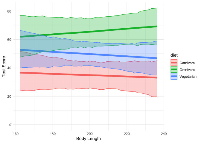
Here we can see that indeed, the effect of body length seems to be close to zero for all three diet types.
Hmm…. did adding body length to our model make it better? Since we’re Bayesian statisticians, we can compare distributions of adjusted R2 values for each model to answer this question:
1
2
3
4
5
6
7
8
9
R2 <- data.frame(model.diet=loo_R2(model.diet, summary=FALSE)[,1],
                 model.diet.length=loo_R2(model.diet.length, summary=FALSE)[,1]) %>%
    mutate(diff=model.diet - model.diet.length) %>%
    pivot_longer(model.diet:diff) %>%
    mutate(name=factor(name, levels=c('model.diet', 'model.diet.length', 'diff')))

ggplot(R2, aes(x=name, y=value)) +
    stat_halfeye(point_interval=median_hdi) +
    theme_minimal()
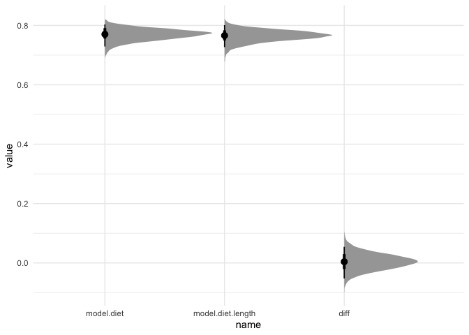
As we can see, both models have an R2 of about 0.75, so adding body length doesn’t seem to help. We can also test their difference using LOO-IC:
1
loo(model.diet, model.diet.length)
1
2
3
4
5
6
7
8
9
10
11
12
13
14
15
16
17
18
19
20
21
22
23
24
25
26
27
28
29
30
31
32
33
34
35
36
37
38
39
40
41
42
## Output of model 'model.diet':
##
## Computed from 4000 by 480 log-likelihood matrix
##
##          Estimate   SE
## elpd_loo  -1832.9 21.6
## p_loo        24.4  4.0
## looic      3665.9 43.2
## ------
## Monte Carlo SE of elpd_loo is NA.
##
## Pareto k diagnostic values:
##                          Count Pct.    Min. n_eff
## (-Inf, 0.5]   (good)     474   98.8%   1097
##  (0.5, 0.7]   (ok)         4    0.8%   230
##    (0.7, 1]   (bad)        2    0.4%   87
##    (1, Inf)   (very bad)   0    0.0%   <NA>
## See help('pareto-k-diagnostic') for details.
##
## Output of model 'model.diet.length':
##
## Computed from 4000 by 480 log-likelihood matrix
##
##          Estimate   SE
## elpd_loo  -1838.1 21.4
## p_loo        30.4  4.1
## looic      3676.2 42.7
## ------
## Monte Carlo SE of elpd_loo is NA.
##
## Pareto k diagnostic values:
##                          Count Pct.    Min. n_eff
## (-Inf, 0.5]   (good)     474   98.8%   1005
##  (0.5, 0.7]   (ok)         5    1.0%   365
##    (0.7, 1]   (bad)        1    0.2%   140
##    (1, Inf)   (very bad)   0    0.0%   <NA>
## See help('pareto-k-diagnostic') for details.
##
## Model comparisons:
##                   elpd_diff se_diff
## model.diet         0.0       0.0
## model.diet.length -5.1       1.8
Again we see that the model without diet does just as well, if not slightly better than, the model with both diet and body length.
Your turn! Try modifying the model above to test whether color is related to testScore, and whether color interacts with diet or bodyLength.
1
2
3
4
5
6
7
8
#Build your model here


#View the output of the model here


#Plot your results below:
Bayesian Multilevel Logistic Regression
Okay, let’s test a new question. Test scores are boring. I actually want to know about which dragons breathe fire. This has way more important practical implications, and is more likely to get me grant funding.
Good news: we have data on fire breathing!
Bad news: It’s a binary variable, so we need to change our model.
With lmer, you need to switch over to the glmer function to gain
access to bernoulli models. But in brms, you just need to specify the
proper noise distribution family:
1
2
3
4
5
logit_model <- brm(breathesFire ~ color + (1+color|mountainRange),
                   data=dragons, file='fire', family=bernoulli,
                   prior=prior(normal(0, 2)))

summary(logit_model, prior=TRUE)
1
2
3
4
5
6
7
8
9
10
11
12
13
14
15
16
17
18
19
20
21
22
23
24
25
26
27
28
29
30
31
32
33
34
35
36
37
38
39
##  Family: bernoulli
##   Links: mu = logit
## Formula: breathesFire ~ color + (1 + color | mountainRange)
##    Data: dragons (Number of observations: 480)
## Samples: 4 chains, each with iter = 2000; warmup = 1000; thin = 1;
##          total post-warmup samples = 4000
##
## Priors:
## b ~ normal(0, 2)
## Intercept ~ student_t(3, 0, 2.5)
## L ~ lkj_corr_cholesky(1)
## sd ~ student_t(3, 0, 2.5)
##
## Group-Level Effects:
## ~mountainRange (Number of levels: 8)
##                       Estimate Est.Error l-95% CI u-95% CI Rhat Bulk_ESS
## sd(Intercept)             0.40      0.27     0.03     1.04 1.00     1346
## sd(color1)                0.35      0.28     0.01     1.04 1.00     1597
## sd(color2)                1.03      0.45     0.39     2.13 1.00     1367
## cor(Intercept,color1)    -0.23      0.48    -0.94     0.77 1.00     2969
## cor(Intercept,color2)     0.15      0.44    -0.72     0.88 1.00     1228
## cor(color1,color2)       -0.07      0.49    -0.88     0.84 1.00     1132
##                       Tail_ESS
## sd(Intercept)             1543
## sd(color1)                1163
## sd(color2)                1103
## cor(Intercept,color1)     2705
## cor(Intercept,color2)     1289
## cor(color1,color2)        1570
##
## Population-Level Effects:
##           Estimate Est.Error l-95% CI u-95% CI Rhat Bulk_ESS Tail_ESS
## Intercept     0.03      0.22    -0.40     0.48 1.00     2196     2212
## color1        2.22      0.26     1.71     2.74 1.00     3108     2349
## color2        0.35      0.42    -0.49     1.17 1.00     1817     1923
##
## Samples were drawn using sampling(NUTS). For each parameter, Bulk_ESS
## and Tail_ESS are effective sample size measures, and Rhat is the potential
## scale reduction factor on split chains (at convergence, Rhat = 1).
Now let’s plot the proportion of dragons that breathe fire by color:
1
2
3
4
5
6
7
8
dragons %>% data_grid(color) %>%
    add_fitted_draws(logit_model, re_formula=NA, scale='response') %>%
    ggplot(aes(x=color, y=.value, fill=color)) +
    stat_halfeye(point_interval=median_hdi, show.legend=FALSE) +
    scale_fill_manual(values=c('blue', 'red', 'yellow')) +
    xlab("Color") +
    ylab("Proportion that Breathes Fire") +
    theme_minimal()
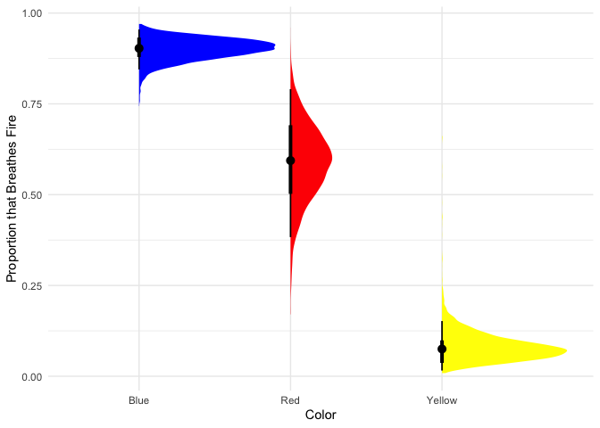
Looks like most blue dragons breathe fire, red dragons are only slightly more likely to breathe fire than not, and few yellow dragons breathe fire.
Your turn! Test whether other variables predict breathesFire.
1
2
3
4
5
#Build your model here:


#Plot your results:
Bayesian Multinomial Regression
One serious advantage of going Bayesian is that you get immediate access to lots of other model types that require significant effort to get from existing Frequentist packages. One example is multinomial regression- this is like logistic regression, but with more than two unordered categories.
Instead of using color to predict body length, let’s see if body length predicts color:
1
2
3
4
5
multi_model <- brm(color ~ bodyLength,
                   data=dragons, file='color', family=categorical,
                   prior=prior(normal(0, 2)))

summary(multi_model, prior=TRUE)
1
2
3
4
5
6
7
8
9
10
11
12
13
14
15
16
17
18
19
20
21
##  Family: categorical
##   Links: muRed = logit; muYellow = logit
## Formula: color ~ bodyLength
##    Data: dragons (Number of observations: 480)
## Samples: 4 chains, each with iter = 2000; warmup = 1000; thin = 1;
##          total post-warmup samples = 4000
##
## Priors:
## b_muRed ~ normal(0, 2)
## b_muYellow ~ normal(0, 2)
##
## Population-Level Effects:
##                     Estimate Est.Error l-95% CI u-95% CI Rhat Bulk_ESS Tail_ESS
## muRed_Intercept         5.62      1.46     2.76     8.52 1.00     3441     3214
## muYellow_Intercept     -7.12      1.67   -10.29    -3.86 1.00     3229     2857
## muRed_bodyLength       -0.03      0.01    -0.04    -0.01 1.00     3399     3110
## muYellow_bodyLength     0.03      0.01     0.02     0.05 1.00     3289     2852
##
## Samples were drawn using sampling(NUTS). For each parameter, Bulk_ESS
## and Tail_ESS are effective sample size measures, and Rhat is the potential
## scale reduction factor on split chains (at convergence, Rhat = 1).
Let’s plot the proportion of dragons of each color by body length:
1
2
3
4
5
6
7
8
9
10
dragons %>% data_grid(bodyLength=seq_range(bodyLength, 100)) %>%
    add_fitted_draws(multi_model, scale='response') %>%
    ggplot(aes(x=bodyLength, y=.value)) +
    stat_lineribbon(aes(color=.category, fill=.category),
                    alpha=0.4, show.legend=FALSE) +
    scale_color_manual(values=c('blue', 'red', 'yellow')) +
    scale_fill_manual(values=c('blue', 'red', 'yellow')) +
    xlab("Body Length") +
    ylab("Probability of Color") +
    theme_minimal()
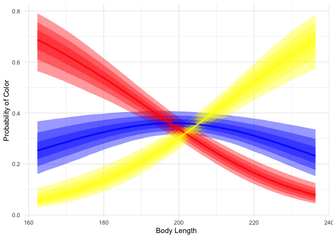
We can see that while short dragons are likely to be red, long dragons are likely to be yellow, and mid-length dragons are likely to be blue.
Bayesian Multilevel Unequal Variances Regression
Another extremely useful example of a model that integrates seamlessly
in brms is unequal variance regression. In our model using diet to
predict test scores, we never checked that the variances in test scores
between dragons with different diets was equal. Since this is an
assumption of that model, it could be bad if that assumption doesn’t
hold. An easy way to get around this in Bayesian regression is to simply
estimate both a mean and a variance for each diet:
1
2
3
4
5
6
model.diet.uv <- brm(bf(testScore ~ diet + (1+diet|mountainRange),
                        sigma ~ diet + (1+diet|mountainRange)),
                     data=dragons, file='diet_uv',
                     prior=set_prior(paste0('normal(0, ', sd(dragons$testScore), ')')))

summary(model.diet.uv, prior=TRUE)
1
2
3
4
5
6
7
8
9
10
11
12
13
14
15
16
17
18
19
20
21
22
23
24
25
26
27
28
29
30
31
32
33
34
35
36
37
38
39
40
41
42
43
44
45
46
47
48
49
50
51
52
53
54
55
56
57
##  Family: gaussian
##   Links: mu = identity; sigma = log
## Formula: testScore ~ diet + (1 + diet | mountainRange)
##          sigma ~ diet + (1 + diet | mountainRange)
##    Data: dragons (Number of observations: 480)
## Samples: 4 chains, each with iter = 2000; warmup = 1000; thin = 1;
##          total post-warmup samples = 4000
##
## Priors:
## b ~ normal(0, 23.0088071104418)
## Intercept ~ student_t(3, 51, 26.1)
## Intercept_sigma ~ student_t(3, 0, 2.5)
## L ~ lkj_corr_cholesky(1)
## sd ~ student_t(3, 0, 26.1)
## sd_sigma ~ student_t(3, 0, 26.1)
##
## Group-Level Effects:
## ~mountainRange (Number of levels: 8)
##                                  Estimate Est.Error l-95% CI u-95% CI Rhat
## sd(Intercept)                       10.78      3.40     6.15    19.37 1.00
## sd(diet1)                            2.33      1.75     0.11     6.64 1.00
## sd(diet2)                            4.47      1.95     1.22     9.15 1.00
## sd(sigma_Intercept)                  0.13      0.09     0.01     0.35 1.00
## sd(sigma_diet1)                      0.22      0.13     0.02     0.54 1.00
## sd(sigma_diet2)                      0.15      0.11     0.01     0.41 1.00
## cor(Intercept,diet1)                 0.03      0.48    -0.85     0.87 1.00
## cor(Intercept,diet2)                 0.74      0.25     0.05     0.99 1.00
## cor(diet1,diet2)                    -0.28      0.45    -0.93     0.74 1.00
## cor(sigma_Intercept,sigma_diet1)     0.08      0.46    -0.80     0.87 1.00
## cor(sigma_Intercept,sigma_diet2)    -0.25      0.46    -0.93     0.73 1.00
## cor(sigma_diet1,sigma_diet2)        -0.42      0.45    -0.96     0.68 1.00
##                                  Bulk_ESS Tail_ESS
## sd(Intercept)                        1699     2357
## sd(diet1)                            1709     2025
## sd(diet2)                            1530     1015
## sd(sigma_Intercept)                  1036     1492
## sd(sigma_diet1)                      1042     1528
## sd(sigma_diet2)                      1094     1931
## cor(Intercept,diet1)                 3565     2868
## cor(Intercept,diet2)                 2202     2767
## cor(diet1,diet2)                     3147     2916
## cor(sigma_Intercept,sigma_diet1)     2046     2306
## cor(sigma_Intercept,sigma_diet2)     2546     2460
## cor(sigma_diet1,sigma_diet2)         2248     2533
##
## Population-Level Effects:
##                 Estimate Est.Error l-95% CI u-95% CI Rhat Bulk_ESS Tail_ESS
## Intercept          49.20      4.04    41.03    57.44 1.00     1289     1798
## sigma_Intercept     2.39      0.08     2.25     2.54 1.00     2288     2156
## diet1             -15.53      1.62   -18.63   -12.27 1.00     1900     2589
## diet2              15.41      2.09    11.08    19.37 1.00     1885     2209
## sigma_diet1         0.16      0.11    -0.05     0.41 1.00     2260     2164
## sigma_diet2         0.02      0.09    -0.14     0.22 1.00     2306     1814
##
## Samples were drawn using sampling(NUTS). For each parameter, Bulk_ESS
## and Tail_ESS are effective sample size measures, and Rhat is the potential
## scale reduction factor on split chains (at convergence, Rhat = 1).
Let’s plot the predicted mean and standard deviation of test scores by diet:
1
2
3
4
5
6
7
8
9
draws <- dragons %>%
    data_grid(diet) %>%
    add_fitted_draws(model.diet.uv, dpar='sigma', re_formula=NA)

draws %>%
    ggplot(aes(x=diet, y=.value)) +
    stat_halfeye(point_interval=median_hdi) + ylim(0, NA) +
    xlab("Diet") + ylab("Test Score") +
    theme_minimal()

1
2
3
4
5
draws %>%
    ggplot(aes(x=diet, y=sigma)) +
    stat_halfeye(point_interval=median_hdi) + ylim(0, NA) +
    xlab("Diet") + ylab("Std Deviation Test Score") +
    theme_minimal()

It looks like the variation in test scores might be smaller for vegetarian dragons than for carnivorous dragons, though the difference is small. Does this unequal variance model do better than our old model?
1
loo(model.diet, model.diet.uv)
1
2
3
4
5
6
7
8
9
10
11
12
13
14
15
16
17
18
19
20
21
22
23
24
25
26
27
28
29
30
31
32
33
34
35
36
37
38
39
40
41
42
## Output of model 'model.diet':
##
## Computed from 4000 by 480 log-likelihood matrix
##
##          Estimate   SE
## elpd_loo  -1832.9 21.6
## p_loo        24.4  4.0
## looic      3665.9 43.2
## ------
## Monte Carlo SE of elpd_loo is NA.
##
## Pareto k diagnostic values:
##                          Count Pct.    Min. n_eff
## (-Inf, 0.5]   (good)     474   98.8%   1097
##  (0.5, 0.7]   (ok)         4    0.8%   230
##    (0.7, 1]   (bad)        2    0.4%   87
##    (1, Inf)   (very bad)   0    0.0%   <NA>
## See help('pareto-k-diagnostic') for details.
##
## Output of model 'model.diet.uv':
##
## Computed from 4000 by 480 log-likelihood matrix
##
##          Estimate   SE
## elpd_loo  -1832.7 21.8
## p_loo        42.3  6.7
## looic      3665.3 43.7
## ------
## Monte Carlo SE of elpd_loo is NA.
##
## Pareto k diagnostic values:
##                          Count Pct.    Min. n_eff
## (-Inf, 0.5]   (good)     469   97.7%   627
##  (0.5, 0.7]   (ok)         4    0.8%   176
##    (0.7, 1]   (bad)        7    1.5%   18
##    (1, Inf)   (very bad)   0    0.0%   <NA>
## See help('pareto-k-diagnostic') for details.
##
## Model comparisons:
##               elpd_diff se_diff
## model.diet.uv  0.0       0.0
## model.diet    -0.3       6.6
In this case, it looks like the model without equal variances does about as well as the model with unequal variances. That means we can probably assume equal variances without any problems. But this isn’t always the case, and many research programs are dedicated to explaining why different groups have different variances!
Conclusions
In this tutorial we demonstrated the basics of using brms to run
Bayesian regressions that directly parallel what you’re likely used to
running with lm and lmer. We also demonstrated how to run Bayesian
significant tests with bayestestR and how to plot results from these
models using tidybayes. Though there are many more details to
specifying, running, and interpreting Bayesian models, hopefully this
tutorial convinced you that making the first step is easier than you
imagined!
Convergence
Some parting tips and tricks:
Like with Frequentist multilevel models, one of the biggest concerns
with convergence is whether you have enough data for your model
structure. Specifically, you need enough observations for every
combination of population-level and group-level effect in order for your
model to be well-defined. Unlike lmer, brms will try to fit a model
even if you don’t have enough data. But in this case, you will either
get unstable results, or your model will only be informed by your
priors.
There are a few different convergence problems that brms will tell you
about, however. If Rhat for any of your parameters is greater than
1.1, then your model has not converged and the samples from your model
don’t match the true posterior. Here, brms will likely instruct you to
increase the number of samples and/or turn on thinning, which reduces
the autocorrelation between samples. If you have divergent transitions,
then brms will tell you to increase the adapt_delta parameter, which
lowers the step size of the estimator. Finally, you might get warnings
about max_treedepth or ESS, both of which brms will give you
recommendations for.
In my experience, however, one of the main reasons that these warnings
might persist is that your priors are underspecified. If you have flat
or extremely wide priors, then brms has to search a massive parameter
space to find the most likely values. But if you constrain your prior to
a reasonable degree, not only will your model fit faster, but it will
also have less convergence issues. No matter what, you want to make sure
that your priors truly reflect your expectations and that your results
aren’t too heavily influenced by your specific choice of prior.