Shenyang Huang Follow PhD Student in Cognitive Neuroscience at Duke University working with Dr. Roberto Cabeza, Dr. Simon Davis, and Dr. Felipe De Brigard.

MATLAB basics

This workshop is written in MATLAB live script: 2022-01-28-matlab-basics.mlx

Why are we even here?
Getting licensed
Working environment
Data types and operations
Conditional Statements and Loops
Functions
How to understand/debug existing code
Local functions must be decalred in the last code section, so here it is

1. Why are we even here?

MATLAB is good in several aspects: it has a useful working environment, operates fast on matrices, has abundant toolboxes and legacy code, and can run on different operation systems (Windows, macOS, Linux). The last point is relevant to the choice of fMRI analysis packages (e.g., SPM vs. FSL, AFNI).

But, MATLAB is also bad and ugly in several ways. It’s not free. It’s giant in size. It’s has some weird features;

2. Getting licensed

Like driving a car or buying a gun, you need a license to use MATLAB, which is NOT free, but Duke does have an institution license that allows you to activate MATLAB (and a bunch of other stuff) with your Duke email here. Check https://software.duke.edu/node/130 or https://oit.duke.edu/help/articles/kb0023255.

In case you want to try out MATLAB without installing it yet, you can use MATLAB Online: https://matlab.mathworks.com/. Note that the online version also requires an active license.

3. Working environment

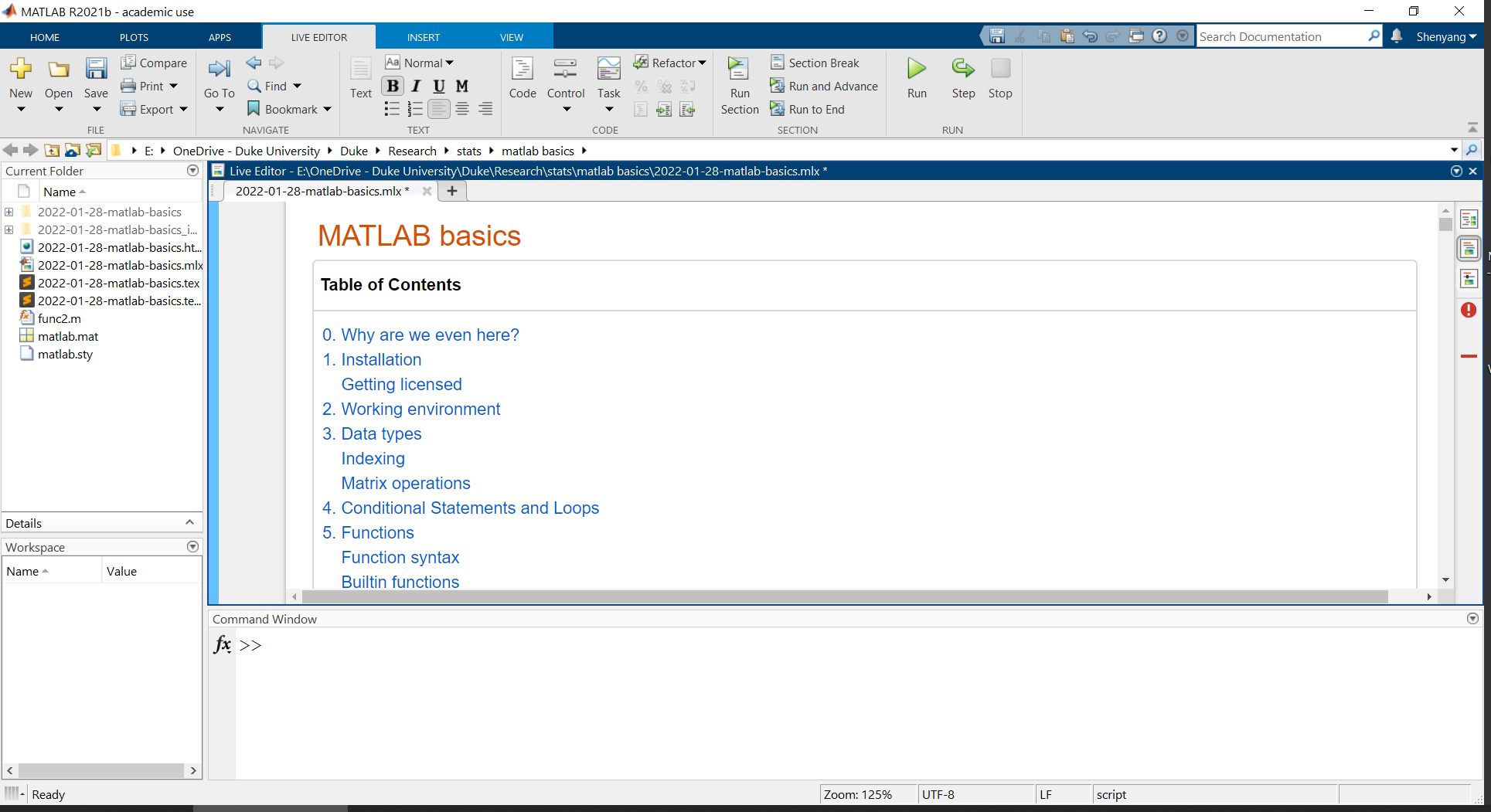
Current Folder: shows things in the current working directory (which is a subset of things on Path; more about Path later)

Workspace: MATLAB’s “working memory” for convenient operations

Command Window: tells MATLAB what it needs to do, and it gets the job done

Editor: essentially a text editor with many useful features, including syntax highlighting, pop-up warnings, and breakpoints for debugging

And, all sorts of buttons up top

4. Data types and operations

Let’s start with the basic data types in MATLAB. This is not a comprehensive list, but you can learn more data types here: https://www.mathworks.com/help/matlab/data-types.html.

Numeric types

% double	Double-precision arrays (64-bit) <-- MATLAB default
% single	Single-precision arrays (32-bit)
% int8	    8-bit signed integer arrays
% uint8	    8-bit unsigned integer arrays
% ...
% for example:
class(1) % use the function class to check data types

ans = 'double'

% use space or comma to separate columns
% use semicolon to separate rows
% use square brackets [ ] to put things together
a = [1    2,    3;
    .5    inf   nan] % this is a 2 x 3 double array

a = 2x3    
    1.0000    2.0000    3.0000
    0.5000       Inf       NaN

% note the two special numbers: Inf and NaN (not a number)
class(a) % the data type is still 'double'

ans = 'double'

Characters and Strings

% use single quotes for characters
char1 = 'a';
char2 = 'abc';
% use double quotes for strings
string1 = "a";
string2 = "abc";
% check data types
class(char1);
class(string1);
% difference
length(char2)

ans = 3

length(string2)

ans = 1

% if we want to concatnate different things
[char1 char2] % correctly concatenated character array

ans = 'aabc'

string1 + string2 % correctly concatenated strings

ans = "aabc"

char1 + char2 % data type converted to numeric for addition

ans = 1x3    
   194   195   196

[char1 string2] % character coerced to string

ans = 1x2 string    
"a"          "abc"

Tables

% values in one column need to be of the same type
% columns can be created with dot indexing names
T = table;
T.col1 = [1; 2];
T.col2 = ["hello"; "world"];
try; T.col3 = 1; catch err; disp(err); end

  MException with properties:

    identifier: 'MATLAB:table:RowDimensionMismatch'
       message: 'To assign to or create a variable in a table, the number of rows must match the height of the table.'
         cause: {}
         stack: [1x1 struct]
    Correction: []

T

	col1	col2
1	1	“hello”
2	2	“world”

Cell Arrays

% use curly brackets to put together things of different sizes and types
C = {42, "abcd"; 'efg', [1 2 3]}

	1	2
1	42	“abcd”
2	‘efg’	[1,2,3]

C(1) % retrieves the cell 

ans = 
    {[42]}

C{1} % retrieves content within the cell

ans = 42

Structures

% group data using fields
% each field can be of any data type, including structures
S = struct;
S.field1_struct = struct;
S.field2_cell = C;
S.field3_table = T;
S.field4_char = char1;
S

S = 
    field1_struct: [1x1 struct]
      field2_cell: {2x2 cell}
     field3_table: [2x2 table]
      field4_char: 'a'

Indexing

% Arrays are efficient, but make sure you access the data in the array in
% the correct fashion

% double arrays are indexed with parentheses
a = [1 2 3; 4 5 6]; % 2 x 3 double array
a(1, 2) % row 1, column 2

ans = 2

a(1:end, 2) % all rows, column 2, equivalent to [2;5]

ans = 2x1    
     2
     5

a(2, :) % row 2, all columns, equivalent to [4 5 6]

ans = 1x3    
     4     5     6

% here's something that may seem odd
a(4) % 4th entry in the (straightened) array

ans = 5

a(:) % full straightened array

If you know R or Python, you may know that array data is stored in the row-wise fashion. In contrast, MATLAB does so differently; array data are stored column-wise, even though arrays are easily defined row-wise. That is to say, in MATLAB, adjacent values in the same column, not the same row, are stored in adjacent positions in computer memory.

This feature of MATLAB influences code efficiency depending on the order in which arrays are created or accessed.

% update each entry of the matrix in different orders
% use the functions tic toc to time the operation
tic; m1 = nan(1000);
for i=1:1000; for j=1:1000
        m1(i,j) = 1;
end; end; fprintf('Update in rows: \n   '); toc

Update in rows: 
   Elapsed time is 0.012881 seconds.

tic; m2 = nan(1000);
for j=1:1000; for i=1:1000
        m2(i,j) = 1;
end; end; fprintf('Update in columns: \n   '); toc

Update in columns: 
   Elapsed time is 0.011935 seconds.

tic; m3 = [];
for i=1:1000
    m3 = [m3; ones(1000,1)];
end
fprintf('Assign values row-wise: \n   '); toc

Assign values row-wise: 
   Elapsed time is 1.385312 seconds.

tic; m4 = [];
for i=1:1000
    m4 = [m4, ones(1000,1)];
end
fprintf('Assign values column-wise: \n   '); toc

Assign values column-wise: 
   Elapsed time is 2.278768 seconds.

b = nan(1000);
c = nan(1000);
tic
for i=1:1000
    b(i,:) = ones(1000,1);
end
fprintf('Assign values row-wise, with preallocation: \n   '); toc

Assign values row-wise, with preallocation: 
   Elapsed time is 0.015013 seconds.

tic
for i=1:1000
    c(:,i) = ones(1000,1);
end
fprintf('Assign values column-wise, with preallocation: \n   '); toc

Assign values column-wise, with preallocation: 
   Elapsed time is 0.011517 seconds.

tic; f = ones(1000); fprintf('Assign values use the native function: \n   '); toc

Assign values use the native function: 
   Elapsed time is 0.002986 seconds.

Take home message: try to index arrays as explicitly as possible and try to pre-allocate space for big arrays.

Matrix operations

% addition and subraction (+ -)
[1 2 3] + [4 5 6]

ans = 1x3    
     5     7     9

try; [1 2 3] + [4 5]; catch err; disp(err); end

  MException with properties:

    identifier: 'MATLAB:sizeDimensionsMustMatch'
       message: 'Arrays have incompatible sizes for this operation.'
         cause: {}
         stack: [1x1 struct]
    Correction: []

[1,2,3] + [4;5] % Note the difference between , and ;

ans = 2x3    
     5     6     7
     6     7     8

% in this case MATLAB automatically populates the missing entries
% and the output is equivalent to that of the following:
[1,2,3; 1,2,3] + [4 4 4; 5 5 5]

ans = 2x3    
     5     6     7
     6     7     8

% multiplication
%%% matrix multiplication (*)
rng(2022)
A = randi(9,2,3)

A = 2x3    
     1     2     7
     5     1     5

B = randi(9,2,2)

B = 2x2    
     9     9
     6     7

C = randi(9,2,2)

C = 2x2    
     8     8
     8     9

% A*B is not allowed due to dimension mismatch, while B*A and B*B are.
B*A

ans = 2x3    
    54    27   108
    41    19    77

B*B

ans = 2x2    
   135   144
    96   103

%%% element-wise multiplication (.*)
%%% this is perhaps more common in everyday use
B.*C % every entry in B is multiplied by every corresponding entry in C

ans = 2x2    
    72    72
    48    63

[1,2].*B % same as in addition, MATLAB automatically populates multiplier here

ans = 2x2    
     9    18
     6    14

[1;2].*B % output is different from that of the previous line

ans = 2x2    
     9     9
    12    14

2.*B % this can be abbreviated as 2*B, but it's still an element-wise multiplication

ans = 2x2    
    18    18
    12    14

5. Conditional Statements and Loops

Conditional statements are designed to execute code based on certain criteria; for example, we may want to print out values that are >2 SD away from the mean to check for outliers.

% There are two ways to write conditional statements
x = 5;
if x > 10
    fprintf('x is greater than 10 \n')
elseif x > 5
    fprintf('x is greater than 5 \n')
elseif x == 5
    fprintf('x is exactly 5 \n')
else 
    fprintf('x is smaller than 5 \n')
end

x is exactly 5

% Three logical operators, &, |, ~
1==1 & 1==2

ans = 
   0

1==1 | 1==2

ans = 
   1

~(1==1)

ans = 
   0

% if there are specific values with which you wish to compare with the variable,
% instead of using x==5, you can use the switch-case syntax
switch x
    case 10
        fprintf('x is exactly 10 \n')
    case 5
        fprintf('x is exactly 5 \n')
    case '1'
        fprintf("x is a character array '1' \n")
end

x is exactly 5

Loops are designed to allow repeated execution of code sections. There are definite loops, where the (maximum) number of iterations is pre-determined, and indefinite loops, where that number is uncertain.

% definite loop
for i = 1:5
    disp(i)
end

% indefinite loop
i = 1;
while i < 6 % note that this is a condition
    disp(i)
    i = i+1;
end

% you can also combine conditional statements with loops
% this does the exact same thing as above
i = 1;
while true
    if i>=6; break; end
    disp(i)
    i = i+1;
end

for i = 1:10
    if mod(i, 2) == 0 % if i is even
        continue % skip to the next iteration
    end
    if i == 6 % note that this line will NOT be evaluated
        break % terminate the entire loop prematurely
    end 
    disp(i)
end

6. Functions

In mathematics, a function is a mapping from an input to an output,

f(x) = sin(x)

, where the output is fixed given the input. In MATLAB (and programming languages in general), a function is a self-contained set of operations that accomplishs a specific task by taking your input, filling out the unspecified parameters with default values, and generating some output.

Built-in functions

These are the most basic functions that comes with MATLAB. We’ve come across some of them in the examples above.

% clear % removes variables from Workspace
% clc % cleans Command Window (but not command history)
% ls % shows content in current directory
% dir % shows content in current directory
% save
% load
% mkdir % make directory (folder)
% double; string; table; cell; struct; 

Function syntax

For all functions in MATLAB, you can call them in two ways: command syntax or function syntax.

% char is a function that generates a character array from the input array
% compare the following ways to use the same function on seemingly same inputs
char duke

ans = 'duke'

char 'duke'

ans = 'duke'

char "duke" 

ans = '"duke"'

char("duke")

ans = 'duke'

char('duke')

ans = 'duke'

try; char(duke); catch err; disp(err); end
duke = [100 117; 107 101]; char(duke)

ans = 
    'du'
    'ke'

double duke

ans = 1x4    
   100   117   107   101

As you may notice, there are two equivalent ways to call a function on the same character array:

function input        % <-- Command Syntax
function('input')     % <-- Function Syntax

Some built-in functions are basic enough (e.g., clear, clc, save, load) that you can safely use them using the command syntax for simplicity. However, the function syntax is much preferred for the following reasons:

% 1. You can use long/repeated input values as variables for convenience
char('a very long character array'); char('a very long character array'); char('a very long character array');
% vs
var = 'a very long character array'; char(var); char(var); char(var);

% 2. Not all input values are character arrays.
% sqrt 100;
% sqrt('100');
sqrt(100);

% 3. Output from command-syntax function calls cannot be stored as variables
% A = char duke;  <-- syntax error
B = char('duke');
B

B = 'duke'

User-declared functions

In addition to built-in functions from MATLAB, you can also use user-decalred functions. This can be down in two ways: 1) create a local function within the script or 2) create a separate function script.

Local functions

Unlike in most other programming languages like Python and R where functions need to be defined before they are called, functions in MATLAB must be defined at the end of the script, probably because MATLAB tries to optimize all the code before execution for speed.

% Suppose we want to switch the order of the first two inputs and take the
% square of the third, and repeat the exact same set of procedures many times,
% it may be convenient if we can "set of procedures"

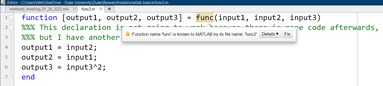
% This declaration is not going to work because there is more code afterwards,
% but I have another exact declaration at the end.

% function [output1, output2, output3] = func(input1, input2, input3)
% output1 = input2;
% output2 = input1;
% output3 = input3^2;
% end
[a, b, c] = func("d", 'hahaha', 5)

a = 'hahaha'
b = "d"
c = 25

Function files

If the function declaration is fairly complicated or is going to be used multiple times in different scripts, it may be convenient to create a function file separate from the script.

% in the current directory, there is a MATLAB script named func2.m which
% contains the exact same function declaration as func
[a, b, c] = func2("d", 'haha', 5)

a = 'haha'
b = "d"
c = 25

Toolboxes

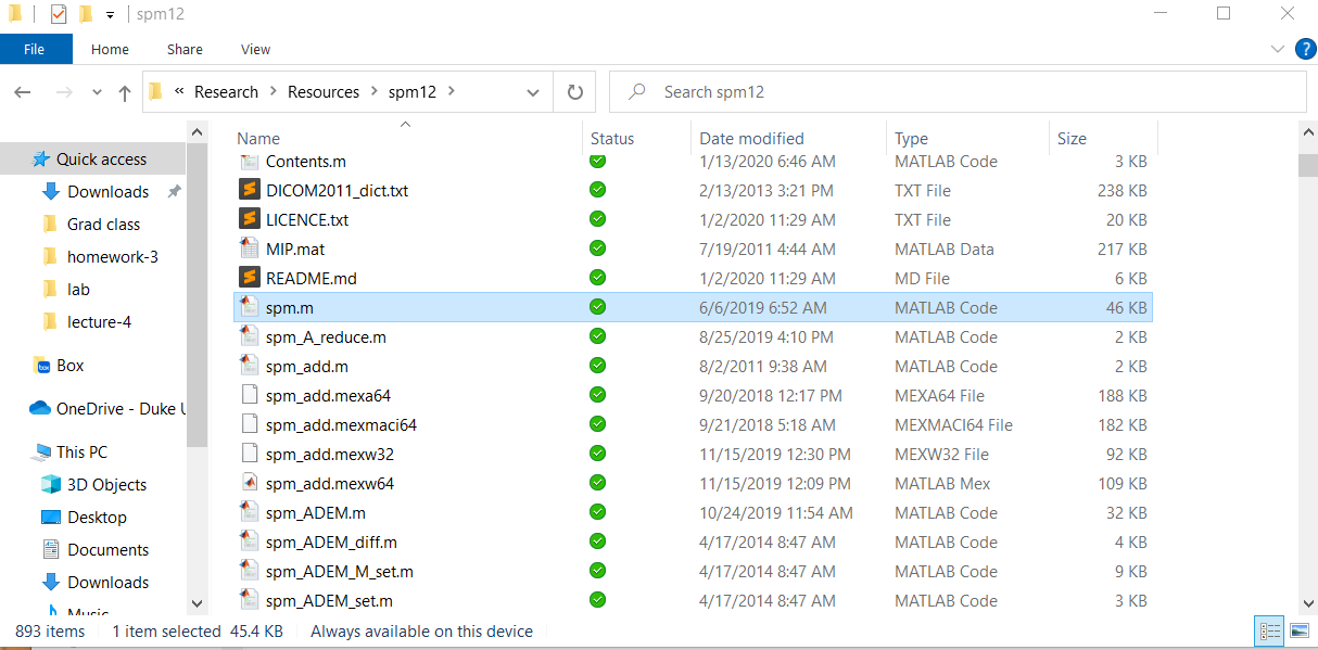
MATLAB toolboxes are (mostly) collections of user-declared functions. Let’s take SPM (Statistical Parametric Mapping, https://www.fil.ion.ucl.ac.uk/spm/)) as an example. Once you download the toolbox from the SPM website, you will get a (zipped) folder containing things like MATLAB scripts, subfolders, and explanatory documents. In the screenshot you can see a MATLAB script called ‘spm.m’, which is a MATLAB function script like the ones we made just now.

Let’s try calling the spm function.

rmpath('E:\OneDrive - Duke University\Duke\Research\Resources\spm12'); % let me make sure spm is NOT on path
try; spm; catch err; disp(err); end

  MException with properties:

    identifier: 'MATLAB:UndefinedFunction'
       message: 'Unrecognized function or variable 'spm'.'
         cause: {}
         stack: [1x1 struct]
    Correction: []

That did not work. Why? Because MATLAB does not know where this function is. To remedy, you can do one of the following:

Move the SPM folder into your current working directory.
Make the SPM folder your working directory.
Use the function ‘addpath’ to add the SPM folder to MATLAB’s path whenever needed. (This operation is temporary, so you will need to do so every time you start a new MATLAB program.)
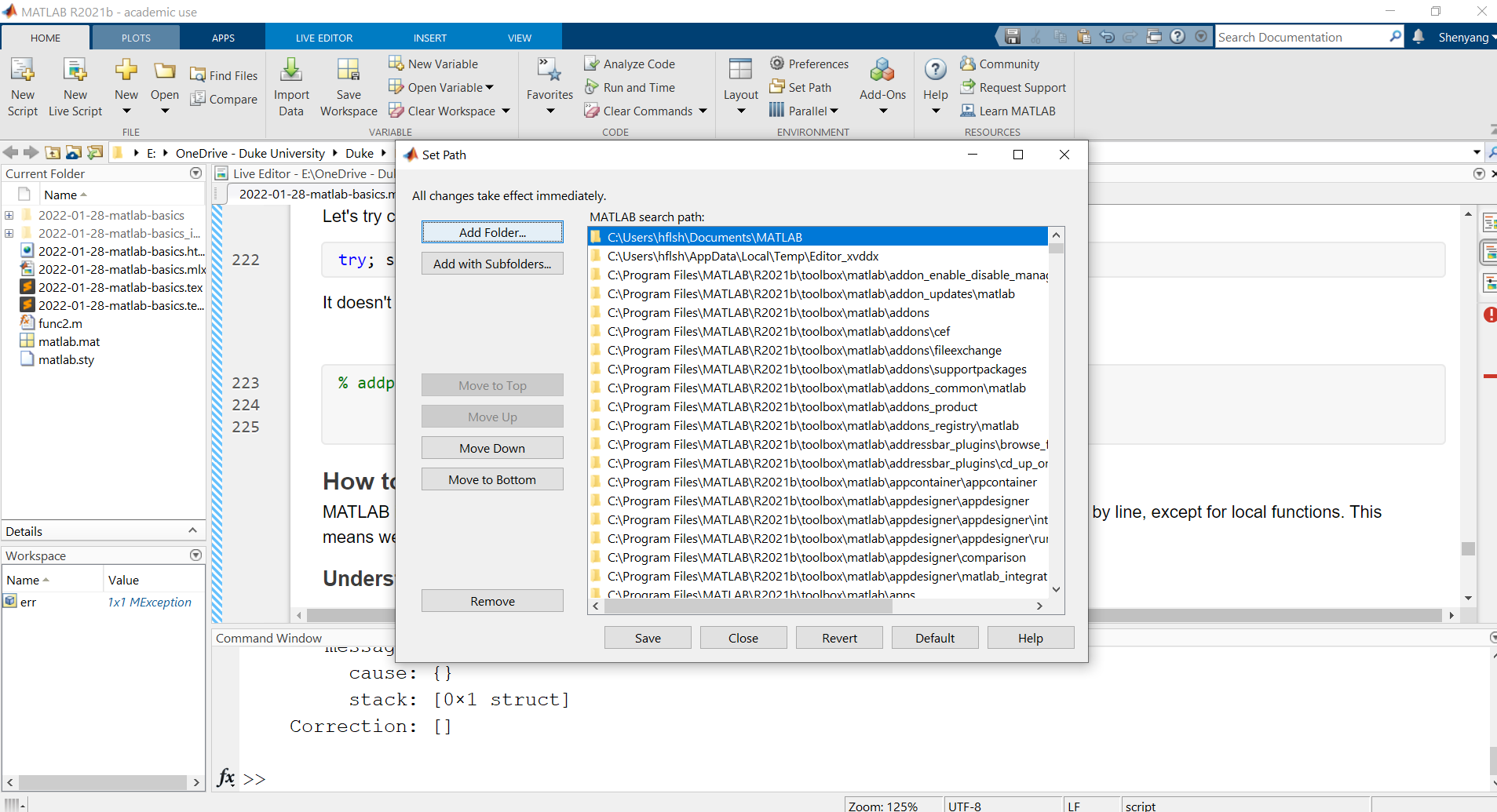
Click on Set Path and add the SPM folder from there. (This operation is permanent, so you only need to do so once unless you reinstall MATLAB.)

addpath('E:\OneDrive - Duke University\Duke\Research\Resources\spm12');
% check where the spm.m function script is, using a built-in function which 
which spm

E:\OneDrive - Duke University\Duke\Research\Resources\spm12\spm.m

% then try calling spm again
spm

7. How to understand/debug existing code

MATLAB is an interpreted programming language–like R and Python, meaning that its code runs line by line, except for local functions. This means we can pause code execution at any point to look at intermediate processes.

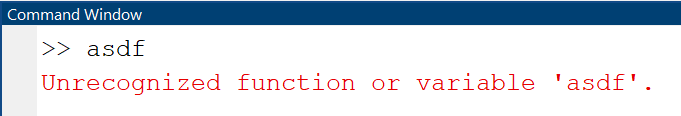
Understanding error messages

When your code execution encounters an error, it will be printed in red in the Command Window, like so:

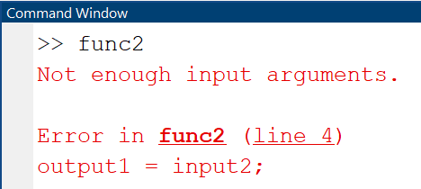
Sometimes the error involves an operation or a function, and you will see that func2 is bolded and underlined. You can click on it to open the help page, or click on the line number to see the exact line of code where the error occured.

Using breakpoints

Breakpoints are a useful way to pause the code at the exact place you want (usually a few steps before the actual error) so that you can pace carefully to investigate the source of the error. It’s a little hard to but you can check

a=1;
b="test";
% c=func2(a, b); % missing one input argument

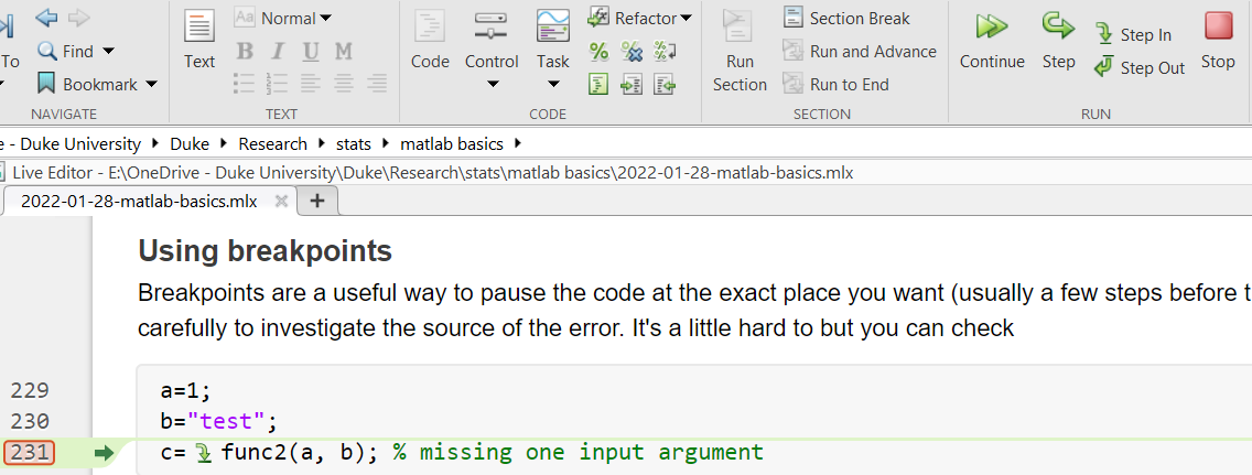
In this example, I set a breakpoint on line 231, and the code paused right before the function call which would have induced an error due to missing input argument. Notice that on the toolbar we have several different buttons that would allow you to execute all the way (Continue), execute the next line only (Step), go into the function that is called (Step in), or give up (Stop).

More ways to use breakpoints here: https://www.mathworks.com/help/matlab/matlab_prog/set-breakpoints.html.

Try-Catch

Sometimes it may be impractical to fully–we may have to use the same script for multiple conditions or multiple subjects, some of which may contain corrupt data that produce errors and make MATLAB stop prematurely. In those cases, it may be preferable to allow MATLAB to keep a record of those errors, ignore them, finish everyone else.

for i={1 2 "3" 0}
    i = i{1};
    try
        5/i
    catch err
        disp(err.message)
    end
end

ans = 5
ans = 2.5000
Arguments must be numeric, char, or logical.
ans = Inf

Finally, some common errors

Incorrect data types.

SPM only accepts character arrays (and sometimes cells containing character arrays), but not strings.
Indexing cell arrays with [ ] or { }. }

Special numbers: 0, inf, nan

They may not cause explicit MATLAB errors at the level of code execution; however, you will get erroneous results
e.g., mean([1 2 3 nan]) or mean([1 2 3 inf]) when you should ignore those entries since they indicate missing data.

Path

MATLAB cannot find the required function before it’s added to path, or if the function name is incorrect.
The path to data or function is spelled incorrectly, e.g., missing a slash ‘/’.

8. Local functions must be decalred in the last code section, so here it is

function [output1, output2, output3] = func(input1, input2, input3)
output1 = input2;
output2 = input1;
output3 = input3^2;
end

That concludes our basic introduction to MATLAB. I hope it could save y’all some time trying to write up your own script or understand and debug legacy code from others. Like Kevin mentioned, we’ll have a hands-on session next week, Feb 4th, during which we can walk through some of the example code in greater depth. Feel free to bring your own code too!

28 Jan 2022

programming

« Blogging with markdown Unconvoluting convolutions - an introduction and applications to neuroscience »

Duke Institute for Brain Sciences Methods Meetings