
Neural Networks
Hello! I hope you’re doing well. Today we have a tutorial on ~ neural networks ~
What exactly is a neural network? We’re not talking about our brains we’re talking about computers. At its core, a neural network is a lot of math that we usually can’t do by hand, and can’t really understand. The motivation behind this math is that we want to model relationships between data and outcomes. In this group we’ve seen a lot of examples of how to do this, primarily focusing on things like regression. The basics of neural networks actually share a lot with logistic regression, but we’ll get to that. The thing is, these models assume a linear or simply transformed linear relationship between data and outcomes. However, this doesn’t exist in a lot of cases, especially when dealing with real-world stimuli. For example, the transformations between images (pixels), categories, and neural activity are incredibly complex, and neural networks give us a way to model the transformations. With complex masses of data, neural networks give us arbitrarily complex models that we can fit to whatever data we have.
Logistic Regression and Perceptrons
We’ll get to the super complex models, but the neural network has humble beginnings. Its most basic form was actually inspired by neurons (hence the name neural networks), and was known as the perceptron (shown below).


The basic premise is simple - you have a bunch of inputs \((x_1,...,x_M)\), weighted by their importance \((w_1,...,w_M)\), which are combined in y and eventually lead to some output. Usually there’s some nonlinearity in y - originally this was either the sigmoid function or step function, to constrain outputs to be between zero and one. Just like a neuron! Differently weighted inputs combine in the soma, there’s some nonlinearity applied, then the neuron either fires or doesn’t fire (yes it’s more complicated than that but this is a simple model okay).
For the more math-y way, we can write this as output = \(y(\sum_{i=1}^m x_i w_i + b)\), or \(y(XW + b)\) in matrix notation.
You may notice, that this is also pretty similar to linear and logistic regression so far, depending on what happens in y! When y is the identity function (\(f(x) = x\)) this is just linear regression, and when \(y\) is the logit function this is logistic regression. So originally, the difference was just in the nonlinearity applied. Since the nonlinearity applied was typically to bound the response between 0 and 1 for classification purposes, a good original comparison is to logistic regression. So let’s do a quick example comparing the two! (btw this will all be in Python)
To start off, we’ll just load in some data! This is going to use the dragon data from previous examples in the class, plus a couple of modifications for illustration purposes. We’re going to add an additional category indicating number of toes, and we’re going to change the length category a bit to make these two groups (approximately) linearly separable.
1
2
3
4
import numpy as np
from sklearn.linear_model import LogisticRegression
# we will use these packages later
1
2
3
4
5
6
7
8
9
10
11
12
13
14
15
16
17
18
19
20
from google.colab import drive
import pandas as pd
#pandas basically turns things into tables like you'd see in R
drive.mount('/content/drive', force_remount=True)
data_dir = "drive/MyDrive/2020-10-21-dragon-data.csv"
d_dat = pd.read_csv(data_dir)
ntoes = np.array([5,6,7,8,9,10,22])
p_fire = np.array([0.3,0.25,0.2,0.15,0.07,0.02,0.01])
p_nofire = np.flip(p_fire)
d_dat['numberToes'] = 0
d_dat.loc[d_dat['breathesFire'] == 1,'numberToes'] = np.random.choice(ntoes,size=(sum(d_dat['breathesFire']),),p=p_fire)
d_dat.loc[d_dat['breathesFire'] == 0,'numberToes'] = np.random.choice(ntoes,size=(sum(1 - d_dat['breathesFire']),),p=p_nofire)
d_dat.loc[d_dat['breathesFire'] == 1,'bodyLength'] -= 30
d_dat.loc[d_dat['breathesFire'] == 0,'bodyLength'] += 30
1
Mounted at /content/drive
1
list(d_dat.columns)
1
2
3
4
5
6
7
['testScore',
'bodyLength',
'mountainRange',
'color',
'diet',
'breathesFire',
'numberToes']
Since we’re talking about classification problems, let’s see if we can predict whether or not a dragon breathes fire based on the number of toes it has and its body length. In our imaginary world, shorter dragons can breathe fire because their power is more concentrated. and they also have fewer toes because they are reckless and accidentally burn off their toes with their fire so typically have fewer toes. We can see this in the following simple plot.
1
2
3
4
5
6
7
8
9
10
11
12
13
14
import matplotlib.pyplot as plt
ax = plt.gca()
y = np.array(d_dat['breathesFire'])
x = np.array(d_dat[['numberToes','bodyLength']])
ax.scatter(x[y==0,0],x[y==0,1], c = 'r')
ax.scatter(x[y==1,0],x[y==1,1], c = 'b')
ax.set_xlabel('Number of Toes')
ax.set_ylabel('Body Length')
1
Text(0, 0.5, 'bodyLength')
_9_1.png)
Here we’ve plotted our firebreathing dragons as blue and our other dragons as red. We’ll then split our data into training and test data to make sure that we don’t overfit to our training data (which shouldnt be a problem in the case of our data, but good to make sure anyway!)
1
2
3
4
5
6
7
8
9
10
11
12
13
14
15
16
17
18
19
20
21
22
23
24
25
26
27
28
29
30
31
32
33
34
35
36
37
38
39
40
41
42
y_fire = y[y==1]
x_fire = x[y==1,:]
y_non = y[y==0]
x_non = x[y==0,:]
split = 0.6
n_tot = len(y)
n_train = int(n_tot*split)
train_order = np.random.permutation(n_tot)
y_train = y[train_order[0:n_train]]
x_train = x[train_order[0:n_train],:]
y_test = y[train_order[n_train::]]
x_test = x[train_order[n_train::],:]
logistic_model = LogisticRegression().fit(x_train,y_train)
pred = logistic_model.predict(x_test)
pred_all = logistic_model.predict(x)
acc = sum(pred == y_test)/len(y_test)
print('Test Accuracy: %f' %acc)
d = sum(pred[y_test == 1] == 1)/sum(y_test == 1)
fp = sum(pred[y_test == 0] == 1)/sum(y_test == 0)
print('Test Detection rate: %f' %d)
print('Test False positive rate: %f' %fp)
fig, ax = plt.subplots(nrows = 1, ncols=2,sharex = True, sharey = True)
ax[0].scatter(x[y == 0,0], x[y == 0,1],c='r')
ax[0].scatter(x[y == 1,0], x[y == 1,1],c='b')
ax[0].set_xlabel('Number of Toes')
ax[0].set_ylabel('Body length')
ax[0].set_title('Ground truth')
ax[1].scatter(x[pred_all == 0,0], x[pred_all == 0,1],c='r')
ax[1].scatter(x[pred_all == 1,0], x[pred_all == 1,1],c='b')
ax[1].set_title('Predictions')
1
2
3
4
5
6
7
8
9
Test Accuracy: 0.994792
Test Detection rate: 1.000000
Test False positive rate: 0.012048
Text(0.5, 1.0, 'Predictions')
_11_2.png)
Okay! so we do pretty well, only misclassifying a few dragons, since this is pretty much linearly separable. Now let’s compare with a perceptron. With a perceptron, there’s also an sklearn function you could use to demonstrate this but imo it’s useful to see how something simple like this learns its decision boundary.
To fit a perceptron, we use each data point in our training and update our weights after we see each training example. Lets use a step function to classify our data, and say if wx + b >0, y = 1. The following code sets up a class that will be what all perceptrons are (basically what’s going on behind the scenes for the logistic regression case).
The way that we train this algorithm is with something called the Perceptron Learning Algorithm, which just says: if our perceptron misclassifies something, we’re going to change weights in the direction of our misclassification. If we classified a dragon as fire-breathing when its attributes actually suggest non-firebreathing, we will change weights in the negative direction of the attributes, and we’ll do the opposite if we classify a firebreathing dragon as non-firebreathing. We will also include that bias term, and we’ll assume it goes to a data attribute that always takes the value 1, since it’ll be constant for all inputs. Finally, we’re going to add in one more trick to make training a bit more stable - if our input data have really large numbers, changing our weights scaled by input size will cause these values to bounce around a lot. Because of these, we’re going to add a learning rate that decreases over training iterations, basically to say that early on, we’ll learn a lot from our data and move around our decision boundary to the generally correct location, and then later on we’ll fine-tune this boundary until we get to the right solution.
1
2
3
4
5
6
7
8
9
10
11
12
13
14
15
16
17
18
19
20
21
22
23
24
25
26
27
28
29
30
31
32
33
34
35
36
37
38
39
40
41
42
43
44
45
46
47
48
49
50
51
52
53
54
55
56
57
58
59
60
61
62
63
64
65
66
67
68
69
70
71
72
73
74
75
76
import time
class perceptron():
def __init__(self,input_features, weight_change_lim = 0.1):
'''
Building our perceptron - we're just
going to initialize our weights to zero
'''
self.w = np.zeros((input_features,),dtype=np.float32)
self.b = 0.0
self.lim = weight_change_lim
def predict(self, data):
"returns 1 if the data time weights are greater than 0, 0 o.w."
return np.matmul(data,self.w) + self.b > 0
def train(self,trainx,trainy,vis=True,max_iter = 1000):
'''
train using perceptron learning rule:
if decision matches true weight, do nothing
otherwise, update weights as (decision - label)*data
'''
done = False
iter = 0
while not done:
total_change = 0
for d_ind,d in enumerate(trainx):
# predict output based on trained parameters
y_hat = self.predict(d)
y = trainy[d_ind]
if y == y_hat:
# if we predicted the correct outcome,
# don't change anything
weight_change = np.zeros(d.shape)
b_change = 0
else:
# if we were wrong, update weights
# learning rate * (direction of error) * data
weight_change = 1/(iter+1)*(y - y_hat)*d
b_change = 1/(iter+1)*(y - y_hat)*1
self.w += weight_change
self.b += b_change
total_change += sum(abs(weight_change))
if total_change < self.lim:
done = True
if iter >= max_iter:
done = True
if vis:
'''
calculate and plot decision boundary
'''
self.ax = plt.gca()
self.ax.scatter(trainx[trainy==0,0],trainx[trainy==0,1], c = 'r')
self.ax.scatter(trainx[trainy==1,0],trainx[trainy==1,1], c = 'b')
self.ax.set_xlabel('number of toes')
self.ax.set_ylabel('body length')
y_int = -self.b/self.w[1]
slope = -self.w[0]/self.w[1]
self.ax.plot([0,25],[y_int, y_int + slope*25],c='k')
plt.show()
plt.title('plot for iter %d' %iter)
time.sleep(3)
plt.close('all')
iter += 1
Then we can train using the same setup from before!
1
2
3
4
5
6
7
8
9
10
11
12
13
14
15
16
17
18
19
20
21
22
23
24
25
perc = perceptron(input_features=2)
perc.train(x_train,y_train,max_iter = 1500)
yhat = perc.predict(x)
yhat_test = perc.predict(x_test)
acc = sum(yhat_test == y_test)/len(y_test)
print('Test Accuracy: %f' %acc)
d = sum(yhat_test[y_test == 1] == 1)/sum(y_test == 1)
fp = sum(yhat_test[y_test == 0] == 1)/sum(y_test == 0)
print('Test Detection rate: %f' %d)
print('Test False positive rate: %f' %fp)
fig, ax = plt.subplots(nrows = 1, ncols=2,sharex = True, sharey = True)
ax[0].scatter(x[y == 0,0], x[y == 0,1],c='r')
ax[0].scatter(x[y == 1,0], x[y == 1,1],c='b')
ax[0].set_xlabel('Number of Toes')
ax[0].set_ylabel('body length')
ax[0].set_title('Ground truth')
ax[1].scatter(x[yhat == 0,0], x[yhat == 0,1],c='r')
ax[1].scatter(x[yhat == 1,0], x[yhat == 1,1],c='b')
ax[1].set_title('Predictions')
_15_0.png)
1
2
3
4
5
6
7
8
9
Test Accuracy: 0.994792
Test Detection rate: 0.990826
Test False positive rate: 0.000000
Text(0.5, 1.0, 'Predictions')
_15_3.png)
As you can see, this does pretty much the exact same performance-wise as logistic regression, if only slightly better.
Multi-class Perceptrons
We can extend this to multi-class classification pretty easily. We basically just stack a bunch of different perceptrons next to each other, then take as our category label the perceptron with the largest output. we’ll use the same update rule as before - if a perceptron is right, don’t change weights, if it’s wrong, change the weights. We have to change our data a little bit, we’re going to use what’s called a one-hot representation for our output - this is just a vector that is all zeros, with a one in the location of the category label. Let’s try this out with our dragon data and predict color from number of toes and body length. We’ll augment the data a little bit (again) to make them easier to separate, just so that we can actually train a (relatively) small neural network on these in a short amount of time.
1
2
3
4
5
6
7
8
9
10
11
12
13
14
15
16
17
18
19
20
21
22
23
24
25
26
27
28
29
30
31
32
33
34
35
36
37
38
39
40
41
42
43
44
45
46
47
48
49
50
51
52
53
54
55
56
57
58
59
60
61
62
63
64
65
66
67
68
69
70
71
72
73
74
75
76
77
78
79
80
81
82
83
84
85
86
87
88
89
90
91
92
93
94
95
96
97
98
class multiclass_perceptron():
def __init__(self,input_shape, n_classes, weight_change_lim = 0.1):
'''
Building our perceptron -
we're just going to initialize our weights to zero
'''
self.n_classes = n_classes
self.w = np.zeros((input_shape,n_classes),dtype=np.float32)
self.b = np.zeros((n_classes,))
self.lim = weight_change_lim
def predict(self,data):
'''
returns the category label predicted by our data & perceptrons
'''
vals = np.matmul(data,self.w) + self.b
max_i = np.argmax(vals,axis=1)
return max_i.astype(np.int8)
def _predict_internal(self, data):
'''
returns a one-hot vector - this will give us a one in the index of the perceptron
with the max value, a zero otherwise
'''
vals = np.matmul(data,self.w) + self.b
max_i = np.argmax(vals,axis=1)
onehot_pred = np.zeros((data.shape[0],self.n_classes),dtype=np.int8)
onehot_pred[:,max_i] = 1
return onehot_pred
def vis_boundaries(self,colors,datax,datay):
'''
calculate and plot decision boundaries
'''
self.ax = plt.gca()
for ii in range(self.n_classes):
self.ax.scatter(datax[datay==ii,0],datax[datay==ii,1],c=colors[ii])
y_int = -self.b[ii]/self.w[1,ii]
slope = -self.w[0,ii]/self.w[1,ii]
self.ax.plot([0,25],[y_int, y_int + slope*25],c=colors[ii])
self.ax.set_xlabel('number of toes')
self.ax.set_ylabel('body length')
self.ax.set_xlim([0,25])
self.ax.set_ylim([50,300])
plt.show()
plt.title('Visualization of decision boundaries')
time.sleep(3)
plt.close('all')
def train(self,trainx,trainy,max_iter = 1000):
'''
train using perceptron learning rule:
if decision matches true weight, do nothing
otherwise, update weights as (decision - label)*data
'''
done = False
iter = 0
while not done:
total_change = 0.0
for d_ind,d in enumerate(trainx):
d = np.expand_dims(d,axis=0)
y_hat = self._predict_internal(d)
y = trainy[d_ind]
y_onehot = np.zeros((1,self.n_classes),dtype=np.int8)
y_onehot[:,y] = 1
for y_ind in range(self.n_classes):
y_tmp = y_onehot[:,y_ind]
yhat_tmp = y_hat[:,y_ind]
if y_tmp == yhat_tmp:
weight_change = np.zeros((d.shape[1],))
b_change = 0
else:
weight_change = np.squeeze(1/(iter+1)*(y_tmp - yhat_tmp)*d)
b_change = 1/(iter+1)*(y_tmp - yhat_tmp)*1
self.w[:,y_ind] += weight_change
self.b[y_ind] += b_change
total_change += sum(abs(weight_change))
if total_change < self.lim:
done = True
if iter >= max_iter:
done = True
iter += 1
1
2
3
4
5
6
7
8
9
10
11
12
13
14
15
16
17
18
19
20
21
22
23
24
25
26
27
28
29
30
31
32
33
34
35
36
37
38
39
40
41
42
43
44
45
y_color = np.array(d_dat['color'])
colors = np.unique(y_color)
y_color_cat = np.zeros(y_color.shape,dtype=np.int8)
for cat, col in enumerate(colors):
y_color_cat[y_color == col] = cat
x[y_color_cat == 1,0] += 7
x[y_color_cat == 1,1] -= 50
x[y_color_cat == 2,1] += 30
x[y_color_cat == 0,0] -= 3
y_train_color = y_color_cat[train_order[0:n_train]]
y_test_color = y_color_cat[train_order[n_train::]]
x_train = x[train_order[0:n_train],:]
x_test = x[train_order[n_train::],:]
cats = np.unique(y_color_cat)
multiperc = multiclass_perceptron(input_shape=2,n_classes=len(cats))
multiperc.train(x_train,y_train_color,max_iter = 1500)
multiperc.vis_boundaries(colors,x_train,y_train_color)
yhat_color = multiperc.predict(x)
yhat_test_color = multiperc.predict(x_test)
acc = sum(yhat_test_color == y_test_color)/len(y_test_color)
print('Test Accuracy: %f' %acc)
fig, ax = plt.subplots(nrows = 1, ncols=2,sharex = True, sharey = True)
for ca in cats:
ax[0].scatter(x[y_color_cat == ca,0], x[y_color_cat == ca,1], c= colors[ca])
ax[0].set_xlabel('Number of Toes')
ax[0].set_ylabel('body length')
ax[0].set_title('Ground truth')
lines = []
for ca in cats:
lines.append(ax[1].scatter(x[yhat_color == ca,0], x[yhat_color == ca,1], c=colors[ca]))
ax[1].set_title('Predictions')
plt.legend(lines,colors)
_19_0.png)
1
2
3
4
5
6
7
Test Accuracy: 0.838542
<matplotlib.legend.Legend at 0x7f6e8710ce10>
_19_3.png)
Please excuse the ugly colors, you can make them better if you want but I’m l a z y. As you can see, this works somewhat. However, we run into a problem here - our data aren’t linearly separable! The boundaries we’re learning aren’t really going to do a good job of classification anymore. So we need a more complicated, nonlinear model.
Multi-Layer Perceptrons
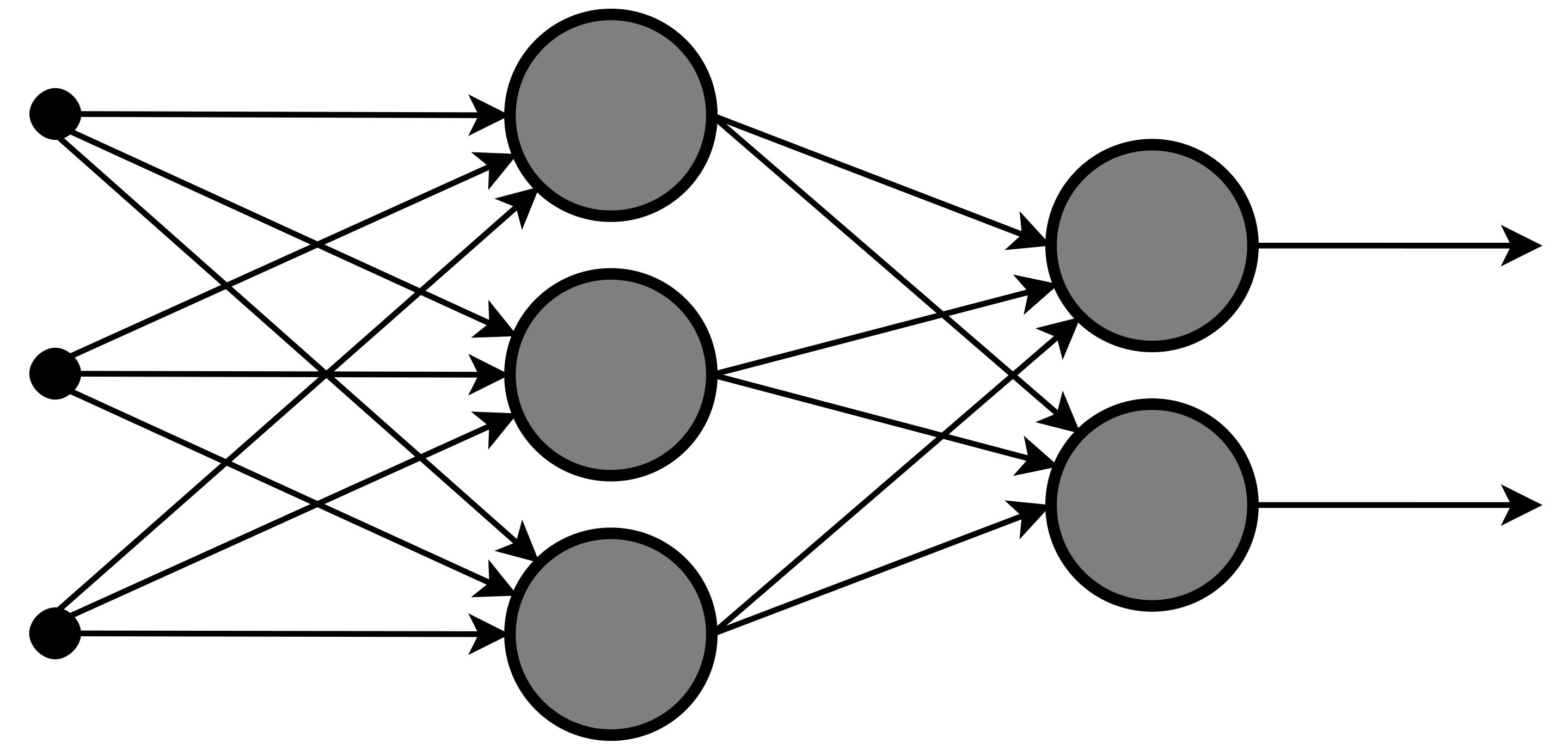
The solution that people came up with is the multilayer perceptron. This is the most basic neural network you could probably have. It’s visualized below, and is the a bunch of these multiclass perceptrons stacked on top of each other.

Here we have a few more terms to introduce. First, we have our input layer. This is just our input features that we want to use to classify (in our case, body length and number of toes). Then we have the hidden layer. This is an arbitrarily large number of learned features. These don’t necessarily have any real-world meaning, but our model has decided that these are an important transformation of the data that make our data easier to classify. The output layer is the same as the output of our previous multiclass perceptron. All of the lines here indicate learned weights.
Deep neural networks are called that because of their depth, or number of hidden layers. More and more layers are stacked together until the network has enough computational power, or enough parameters, to solve the problem you want to solve.
These neural networks also include different activation functions. An activation function is a simple nonlinear function applied after the matrix multiplication we did previously, of weights * data. Some commonly used ones are the sigmoid function (bounds inputs between zero and one), the Rectified Linear Unit (ReLU), which is linear for inputs greater than zero, and zero for inputs less than zero, the leaky ReLU, which scales down inputs less than zero, Softmax, which converts values to probabilities, and others.
With more complex networks, we also get more complex loss functions. A loss function is a way of evaluating the performance of a classifier. In the perceptron learning rule, our loss function was basically a binary right/wrong function.
The typically used loss functions for bigger neural networks are used because because they have two properties: first, they accurately evaluating how well a network is learning. Second, they have a nice derivative. Thanks to the Chain Rule from Math, we can take the derivative of our loss function, and use that to update all of the parameters of our network. I’m not going to get into the math because I don’t like taking derivatives all day, and luckily there are programs that do that for us automatically! The two main ones that people use are pytorch and tensorflow - in research, people tend to use pytorch over tensorflow, which is great because in my opinion pytorch makes more sense than tensorflow.
These programs work with tensors instead of vectors, which are what we’ve been using previously. The way I think about this is saying that a tensor is a generalization of a vector. A point in space is a 1d tensor, a vector is a 2d tensor, a matrix is a 3d tensor, and so on.
I know that’s a lot of information, so below we can find some quick examples of pytorch code. The perceptrons we’ve been working with earlier are known as Fully Connected or linear layers, so we’ll use the fully connected layers here to show the output.
1
2
3
4
5
6
7
8
9
10
11
12
13
14
15
16
17
18
import torch
import torch.nn as nn
## nn.Linear initializes the weights randomly ##
layer1 = nn.Linear(in_features=2,out_features=4)
x1 = torch.tensor(x[0,:],dtype=torch.float32)
y1 = layer1(x1)
y1_t = y1.detach().numpy()
x1_np = x1.detach().numpy()
w_np = layer1.weight.detach().numpy()
b_np = layer1.bias.detach().numpy()
y1_np = np.matmul(w_np,x1_np) + b_np
print(y1_np)
print(y1_t)
1
2
[-59.997787 74.56297 22.336237 95.736145]
[-59.997787 74.56297 22.336237 95.736145]
As we can see, this is just a linear function. Nice! The .detach().numpy() following our tensors indicate two things. First, the .detach() indicates that we should take these tensors out of the computation graph. This is the fancy way that pytorch describes the way it automatically calculates derivatives. The .numpy() turns our tensors into numpy arrays, which are what we’ve been using so far. Let’s take a look at what some of our nonlinearities do.
1
2
3
4
5
6
7
8
9
10
11
12
13
14
nl1 = nn.ReLU()
nl2 = nn.Sigmoid()
nl3 = nn.LeakyReLU()
nl4 = nn.Softmax(dim=0)
y2 = nl1(y1).detach().numpy()
y3 = nl2(y1).detach().numpy()
y4 = nl3(y1).detach().numpy()
y5 = nl4(y1).detach().numpy()
print('ReLU output: ', y2)
print('Sigmoid output: ', y3)
print('Leaky ReLU output: ', y4)
print('Softmax output: ', y5)
1
2
3
4
ReLU output: [ 0. 74.56297 22.336237 95.736145]
Sigmoid output: [8.7759065e-27 1.0000000e+00 1.0000000e+00 1.0000000e+00]
Leaky ReLU output: [-0.59997785 74.56297 22.336237 95.736145 ]
Softmax output: [0.000000e+00 6.376880e-10 1.326857e-32 1.000000e+00]
In our multiclass classification problem from before, we can use whatever we want for our hidden layers, but we might want our final output layer to be a softmax, to indicate the probability that our network thinks a dragon is a certain color, based on its body length and number of toes.
Let’s build a quick network and try this out! We’ll use one hidden layer.
1
2
3
4
5
6
7
8
9
10
11
12
13
14
15
16
17
torch.manual_seed(2021)
# Layer 1: 2 inputs to 10 hidden units
layer1 = nn.Linear(in_features=2,out_features=10)
# Layer 2: 10 hidden units to 20 hidden units
layer2 = nn.Linear(in_features=10,out_features=20)
# Layer 3: 20 hidden units to 1000 hidden units
layer3 = nn.Linear(in_features=20,out_features=1000)
# Layer 4: 1000 hidden units to 3 output units
layer4 = nn.Linear(in_features=1000,out_features=len(colors))
# ReLU: max(0,x)
nonlin1 = nn.ReLU()
# Softmax: turns inputs into a probability distribution
nonlin2 = nn.Softmax(dim=1)
1
2
3
4
5
6
7
8
9
10
11
12
13
14
15
16
17
18
19
20
21
22
23
24
25
26
27
28
29
30
31
def forward_pass(x):
# Takes samples as inputs, passing them through
# each layer, followed by a nonlinearity
x = layer1(x)
x = nonlin1(x)
x = layer2(x)
x = nonlin1(x)
x = layer3(x)
x = nonlin1(x)
x = layer4(x)
out = nonlin2(x)
return out
x1 = torch.tensor(x[25,:],dtype=torch.float32)
x1 = x1.unsqueeze(0)
y1 = y[25]
out1 = forward_pass(x1)
# This is what the output of our network looks like
print(out1)
yhat1 = np.argmax(out1.detach().numpy())
print('Predicted label: ',yhat1)
print('Actual label: ',y1)
print('Predicted color: ',colors[yhat1])
print('Actual color: ', colors[y1])
1
2
3
4
5
tensor([[0.0587, 0.0818, 0.7829]], grad_fn=<SigmoidBackward>)
Predicted label: 2
Actual label: 0
Predicted color: Yellow
Actual color: Blue
Nice! Our network does something! However, it’s not right. Therefore we need some way to train our network. Some way to evaluate the performance of this network. A typical way to do this is with the cross-entropy loss. Cross-entropy loss is defined as the negative log probability of the true label, as output by our network. Basically, this loss function will be really large if our network doesn’t think the true label is very probable. Let’s see how this works!
1
2
3
4
5
6
7
8
def ce_loss(probs,labels):
# takes a set of probabilities and set of labels,
# returns the average negative log probability
# across all labels
return torch.mean(-torch.log(probs[:,labels]))
1
2
3
4
5
cl1 = ce_loss(out1,y1)
print(out1[:,y1])
print(cl1)
1
2
tensor([0.0118], grad_fn=<SelectBackward>)
tensor(4.4433, grad_fn=<MeanBackward0>)
After calculating this for a sample, we then pass the gradient back through the network and update our weights! We’re going to use something called the Adam Optimizer to update our weights - the specifics of that aren’t too important, just know that it’s what most people use to update their network weights based on the gradient from the network.
1
2
3
4
5
6
7
8
9
10
11
12
13
14
15
16
17
18
19
20
21
22
23
from torch.optim import Adam
torch.autograd.set_detect_anomaly(True)
### create list of parameters to optimize ###
parameter_list = [layer1.weight,layer1.bias,\
layer2.weight,layer2.bias,\
layer3.weight,layer3.bias,\
layer4.weight,layer4.bias]
# Initialize an optimizer - this will act on
# the parameter list, passing gradients back
# with the learning rate we specify
optimizer = Adam(parameter_list,lr=2e-4)
# Set the stored gradients to zero
optimizer.zero_grad()
print('Weight before passing the gradient: ',layer1.weight)
# Calculate loss
cl1 = ce_loss(out1,y1)
print('Loss: ', cl1.item())
cl1.backward()
optimizer.step()
print('Weight after passing the gradient back: ',layer1.weight)
1
2
3
4
5
6
7
8
9
10
11
12
13
14
15
16
17
18
19
20
21
22
23
Parameter containing:
tensor([[-0.5226, 0.0189],
[ 0.3430, 0.3053],
[ 0.0997, -0.4734],
[-0.6444, 0.6545],
[-0.2909, -0.5669],
[ 0.4378, -0.6832],
[ 0.4557, -0.5315],
[ 0.3520, -0.1969],
[ 0.0185, -0.2886],
[ 0.4008, 0.3401]], requires_grad=True)
4.443321704864502
Parameter containing:
tensor([[-0.5226, 0.0189],
[ 0.3425, 0.3048],
[ 0.0997, -0.4734],
[-0.6449, 0.6540],
[-0.2909, -0.5669],
[ 0.4378, -0.6832],
[ 0.4557, -0.5315],
[ 0.3520, -0.1969],
[ 0.0185, -0.2886],
[ 0.4003, 0.3396]], requires_grad=True)
1
2
3
4
5
6
7
8
9
10
11
12
13
14
15
16
17
18
19
20
21
22
23
24
25
26
27
28
29
30
31
32
33
34
35
36
37
38
39
40
41
42
43
44
45
46
47
48
49
50
51
52
53
54
55
56
57
58
59
60
61
62
63
64
65
def predict(data):
out_sample = forward_pass(data)
cats = torch.argmax(out_sample,axis=1)
return cats
parameter_list = [layer1.weight,layer1.bias,\
layer2.weight,layer2.bias,\
layer3.weight,layer3.bias,\
layer4.weight,layer4.bias]
optimizer = Adam(parameter_list,lr=2e-4)
# turn data into tensors
x_train_tensor = torch.tensor(x_train,dtype=torch.float32)
y_train_color_tensor = torch.tensor(y_train_color,dtype = torch.long)
x_tensor = torch.tensor(x,dtype=torch.float32)
x_test_tensor = torch.tensor(x_test,dtype=torch.float32)
y_test_color_tensor = torch.tensor(y_test_color,dtype = torch.long)
order = np.random.permutation(len(y_train_color_tensor))
batch_size = 50
batch_ind = 0
for sample_ind in order:
y_sample = y_train_color_tensor[sample_ind]
x_sample = torch.unsqueeze(x_train_tensor[sample_ind,:],0)
# Feed in one sample at a time
out_sample = forward_pass(x_sample)
optimizer.zero_grad()
cl1 = ce_loss(out_sample,y_sample)
cl1.backward()
optimizer.step()
print('Training on samples done!')
y_test_out = predict(x_test_tensor).detach().numpy()
y_out = predict(x_tensor).detach().numpy()
acc = sum(y_test_out == y_test_color)/len(y_test_color)
print('Test Accuracy: %f' %acc)
fig, ax = plt.subplots(nrows = 1, ncols=2,sharex = True, sharey = True)
for ca in cats:
ax[0].scatter(x[y_color_cat == ca,0], x[y_color_cat == ca,1], c= colors[ca])
ax[0].set_xlabel('Number of Toes')
ax[0].set_ylabel('body length')
ax[0].set_title('Ground truth')
lines = []
for ca in cats:
lines.append(ax[1].scatter(x[y_out == ca,0], x[y_out == ca,1], c=colors[ca]))
ax[1].set_title('Predictions')
plt.legend(lines,colors)
1
2
3
4
5
6
7
8
9
Training on samples done!
[0 1 2]
Test Accuracy: 0.760417
<matplotlib.legend.Legend at 0x7f6e35a97d10>
_35_2.png)
Great! we’ve trained our network a little bit! however, it does horribly. Let’s train it some more and see how it does.
1
2
3
4
5
6
7
8
9
10
11
12
13
14
15
16
17
18
19
20
21
22
23
24
25
26
27
28
29
30
31
32
33
34
35
36
37
38
39
40
41
42
43
44
45
46
47
48
49
50
parameter_list = [layer1.weight,layer1.bias,\
layer2.weight,layer2.bias,\
layer3.weight,layer3.bias,\
layer4.weight,layer4.bias]
optimizer = Adam(parameter_list,lr=2e-4)
n_epochs = 25
for ep in range(n_epochs):
order = np.random.permutation(len(y_train_color_tensor))
batch_ind = 0
for sample_ind in order:
y_sample = y_train_color_tensor[sample_ind]
x_sample = torch.unsqueeze(x_train_tensor[sample_ind,:],0)
out_sample = forward_pass(x_sample)
optimizer.zero_grad()
cl1 = ce_loss(out_sample,y_sample)
cl1.backward()
optimizer.step()
yhat = predict(x_train_tensor).detach().numpy()
acc = sum(yhat == y_train_color_tensor.detach().numpy())/len(y_train_color_tensor)
print('Accuracy after epoch %d: %f' %(ep,acc))
print('Training on samples done!')
y_test_out = predict(x_test_tensor).detach().numpy()
y_out = predict(x_tensor).detach().numpy()
acc = sum(y_test_out == y_test_color)/len(y_test_color)
print('Test Accuracy: %f' %acc)
fig, ax = plt.subplots(nrows = 1, ncols=2,sharex = True, sharey = True)
for ca in cats:
ax[0].scatter(x[y_color_cat == ca,0], x[y_color_cat == ca,1], c= colors[ca])
ax[0].set_xlabel('Number of Toes')
ax[0].set_ylabel('body length')
ax[0].set_title('Ground truth')
lines = []
for ca in cats:
lines.append(ax[1].scatter(x[y_out == ca,0], x[y_out == ca,1], c=colors[ca]))
ax[1].set_title('Predictions')
plt.legend(lines,colors)
1
2
3
4
5
6
7
8
9
10
11
12
13
14
15
16
17
18
19
20
21
22
23
24
25
26
27
28
29
30
31
32
33
34
Accuracy after epoch 0: 0.486111
Accuracy after epoch 1: 0.527778
Accuracy after epoch 2: 0.684028
Accuracy after epoch 3: 0.767361
Accuracy after epoch 4: 0.552083
Accuracy after epoch 5: 0.791667
Accuracy after epoch 6: 0.704861
Accuracy after epoch 7: 0.770833
Accuracy after epoch 8: 0.704861
Accuracy after epoch 9: 0.697917
Accuracy after epoch 10: 0.822917
Accuracy after epoch 11: 0.861111
Accuracy after epoch 12: 0.840278
Accuracy after epoch 13: 0.822917
Accuracy after epoch 14: 0.750000
Accuracy after epoch 15: 0.854167
Accuracy after epoch 16: 0.861111
Accuracy after epoch 17: 0.902778
Accuracy after epoch 18: 0.854167
Accuracy after epoch 19: 0.871528
Accuracy after epoch 20: 0.760417
Accuracy after epoch 21: 0.843750
Accuracy after epoch 22: 0.906250
Accuracy after epoch 23: 0.881944
Accuracy after epoch 24: 0.895833
Training on samples done!
Test Accuracy: 0.880208
[0 1 2]
<matplotlib.legend.Legend at 0x7f6e35996110>
_37_2.png)
Yay! This does better! As you can see, we add in a bit of nonlinearity in our decision boundaries, and do even better. The case we have here uses a pretty small amount of data, and goes through it a relatively small number of times, so we don’t do perfectly. However, in theory, if we add in enough layers, enough training examples, and let our network see those examples enough times, we can fit our data perfectly.
One thing you might have noticed is that we aren’t always finding a better network each pass through our data - that’s because we have a lot of parameters, and that makes our loss function very complex as well. We are also only approximating our loss function. The true loss function evaluated the performance of our network over all our data. If we were using that, we’d only pass a gradient backwards through our data after seeing all of it first. However, in practical settings, there’s just too much data for us to do that! So what ends up being good enough is just seeing a subset of our data and taking the gradient over that. The less data we use, the higher variance our gradient will have, which is one of the reasons why just looking at one sample at a time (like we’re doing here) also leads to very high variance gradients and less consistency in accuracy across epochs. You also might notice that we have tons of parameters! They lose their interpretability because there are just s o many. There are some ways to kind of look at what they can mean, but we’re not gonna talk about those today. The main take-away here is that if you care about classification, this will get you a really good classification result.
Okay! so there’s a basic framework for training feed-forward neural networks. Basically that’s how it’s done for a whole lot of neural networks. This can be useful if, say, you want to gather a bunch of behavioral variables (eyetracking, SCR, etc) and introduce some perturbation or have participants make a choice, then see at what point on the trial you start being able to predict the participant response.
More Complex Neural Networks
However, people also use a wide array of other networks for other tasks! We’re not going to implement them but here’s a quick lil sampler with some citations if you’re interested:
First, we have the Convolutional Neural Network. This was used to try and make networks rotation and location invariant. Feedforward networks are great, but let’s say they’re trying to classify digits and are trained only on digits that look right (right side up, not reversed). They won’t be able to classify numbers that are reversed or perturbed in some way, which is a big problem! Convolution fixes this by changing what neural networks learn. A convolution takes a small filter and applies it to patches of the input, acting the same way for each part of the input, rather than learning a separate weight for each part of the input. Here’s how convolutions look, in practice:

for the top example, the red line is the signal and the blue line is the filter. By passing the filter over the red line, we get the black line as output. The same is basically true with the actual image! Passing the filter over different parts of the image produces a feature map, which will differ based on the filter. Stacked layers of convolutions end up giving really impressive performance, actually reaching human performance on many visual recognition tasks! There’s been some investigation into what the learned features tell us, and there have been some comparisons between learned features in DNNs and activation maps in human visual cortex, but what those comparisons mean is up for debate. This paper is a pretty good review of how neural networks have been used in vision science, and as the title suggests it covers positives and negatives of NNs. This type of neural network is also really good for image processing, and has been applied extensively in automated image and pose tracking for rats and monkeys.
Another prominent type of neural network is the Recurrent Neural Network (RNN). The most basic version of this works as a feed-forward neural network, but for sequences. Instead of predicting a category, these take an input from a sequence and try to predict the next element of the sequence. This is used really heavily in text analysis, where you try to predict the next word from the previous few words. It’s also used in simulating actual neural networks in the brain. RNNs are great but tend to forget what happened far into the past, which is where Long Short-Term Memory (LSTM) neural networks come in. These are a subtype of RNNs that have two paths. The first is the classic feed-forward across time. The second keeps early information relatively unmodified across time, such that early information in the sequence is maintained. The diagrams for these are kind of complicated, so I’m not going to put one here.
Neural networks are also used for Reinforcement Learning, which we’ve previously covered using R. This is a whole field on its own so I won’t cover it here, but I will just add that deep learning methods in AI are responsible for some of the big leaps forward in RL performance, being responsible for things like this.
Finally, neural networks are also used in Deep Generative Modeling. There are two main classes here that take the form of Generative Adversarial Networks (GANs) and Autoencoders. GANs are cool because they pit two neural networks against each other. One generative network uses a low-dimensional vector of random values to make samples that the other network will think are real, while one discriminative network tries to get better at distinguishing real samples from fake samples. These are responsible for some of the more realistic looking fake images you might see on the internet - things like these (bottom row of the following image):

They are also really difficult to train! They require a ton of computational power and are kind of unstable, meaning that sometimes after training they just fail completely. The other type, autoencoders, makes somewhat less high quality samples, but is better in terms of the learned representation. Autoencoders take an input, try to compress it to a much lower-dimensional representation, and then try to reconstruct the original image from that low-dimensional representation. These are especially helpful for science in the case of Variational Autoencoders, which implement variational inference in an autoencoder. This uses Bayes’s rule to approximate the low-dimensional representation, leading to a learned representation that contains useful, (approximately) independent information about the input sources.