
Ordinal regression models to analyze Likert scale data
Today I am going to present on an alternative way to analyze Likert scale data by using ordinal regression instead of linear regression. But first, why is it even a problem to use linear regression when analyzing these data?
Here is the thing: in our research, we frequently use Likert scales to get ratings of how participants perceive/evaluate/feel certain features. After collecting the data, we calculate the mean and sd of the items in our scales. However, when doing this we don’t take into account that steps along a Likert scale may not be equivalent in terms of magnitude.
Basically, Likert scales are ordinal scales that offer a way of categorizing the feature measured in a direction (i.e. 1<2<3<4<5…), but do not assume that the magnitude between each step is equal (as opposed to continuous variables). Anyways, when analyzing the data using linear models, we treat an ordinal variable as if it was a continuous one, without accounting for the variance that may result from the fact that the steps in the scale are not equidistant.
My queries about this problem of the Likert scales came from my research trying to get ratings of the severity of wrongdoings when participants were recalling a harm. In a 7-point Likert scale where 1 = not severe at all; and 7 = extremely severe, I can say that my friend lying to me about having an affair with my boss is a 4, and other person can say that their partner lying to them about his plans for the weekend is a 5. This does not necessarily mean that the latter is 25% worse than the former. It just means that one of the harms seems to be more severe than the other.

All this to say that it would be useful to find a way to analyze Likert scale data accounting for differences in the magnitudes within the thresholds of the scales. And here is the answer: Ordinal logistic regressions! So first, we will run the following packages:
1
2
3
4
5
6
library(tidyverse)
library(brms)
library(tidybayes)
library(distributional)

memfor_data_s5 <- read_csv('forgiveness_data.csv')
Just to have a reference, we will first do a regular linear regression:
1
2
3
4
5
6
7
8
9
m.gaussian <- brm(severity_action ~ 1, data=memfor_data_s5)
summary(m.gaussian)

ggplot(memfor_data_s5, aes(x=severity_action)) +
  geom_histogram(aes(y=stat(density)), binwidth=1) +
  geom_line(aes(x=.value, y=y), data=tibble(.value=seq(1, 7, .01)) %>%
              mutate(y=dnorm(.value, mean=mean(memfor_data_s5$severity_action),
                             sd=sd(memfor_data_s5$severity_action)))) +
  theme_classic()
1
2
3
4
5
6
7
8
9
10
11
12
13
14
15
16
17
18
19
20
21
22
23
24
25
26
27
28
29
30
31
32
33
34
35
36
37
38
39
40
41
42
43
44
45
46
47
48
49
50
51
52
53
54
55
56
57
58
59
60
61
62
63
64
65
66
67
68
69
70
71
72
73
74
75
76
77
78
79
80
81
82
83
84
85
86
87
88
89
90
91
92
93
94
95
96
97
98
99
100
101
102
103
104
105
106
107
108
109
110
111
112
113
114
115
116
117
118
##
## SAMPLING FOR MODEL 'bbea73d083f058b5e342facc434b7e40' NOW (CHAIN 1).
## Chain 1:
## Chain 1: Gradient evaluation took 1.5e-05 seconds
## Chain 1: 1000 transitions using 10 leapfrog steps per transition would take 0.15 seconds.
## Chain 1: Adjust your expectations accordingly!
## Chain 1:
## Chain 1:
## Chain 1: Iteration:    1 / 2000 [  0%]  (Warmup)
## Chain 1: Iteration:  200 / 2000 [ 10%]  (Warmup)
## Chain 1: Iteration:  400 / 2000 [ 20%]  (Warmup)
## Chain 1: Iteration:  600 / 2000 [ 30%]  (Warmup)
## Chain 1: Iteration:  800 / 2000 [ 40%]  (Warmup)
## Chain 1: Iteration: 1000 / 2000 [ 50%]  (Warmup)
## Chain 1: Iteration: 1001 / 2000 [ 50%]  (Sampling)
## Chain 1: Iteration: 1200 / 2000 [ 60%]  (Sampling)
## Chain 1: Iteration: 1400 / 2000 [ 70%]  (Sampling)
## Chain 1: Iteration: 1600 / 2000 [ 80%]  (Sampling)
## Chain 1: Iteration: 1800 / 2000 [ 90%]  (Sampling)
## Chain 1: Iteration: 2000 / 2000 [100%]  (Sampling)
## Chain 1:
## Chain 1:  Elapsed Time: 0.024751 seconds (Warm-up)
## Chain 1:                0.027761 seconds (Sampling)
## Chain 1:                0.052512 seconds (Total)
## Chain 1:
##
## SAMPLING FOR MODEL 'bbea73d083f058b5e342facc434b7e40' NOW (CHAIN 2).
## Chain 2:
## Chain 2: Gradient evaluation took 7e-06 seconds
## Chain 2: 1000 transitions using 10 leapfrog steps per transition would take 0.07 seconds.
## Chain 2: Adjust your expectations accordingly!
## Chain 2:
## Chain 2:
## Chain 2: Iteration:    1 / 2000 [  0%]  (Warmup)
## Chain 2: Iteration:  200 / 2000 [ 10%]  (Warmup)
## Chain 2: Iteration:  400 / 2000 [ 20%]  (Warmup)
## Chain 2: Iteration:  600 / 2000 [ 30%]  (Warmup)
## Chain 2: Iteration:  800 / 2000 [ 40%]  (Warmup)
## Chain 2: Iteration: 1000 / 2000 [ 50%]  (Warmup)
## Chain 2: Iteration: 1001 / 2000 [ 50%]  (Sampling)
## Chain 2: Iteration: 1200 / 2000 [ 60%]  (Sampling)
## Chain 2: Iteration: 1400 / 2000 [ 70%]  (Sampling)
## Chain 2: Iteration: 1600 / 2000 [ 80%]  (Sampling)
## Chain 2: Iteration: 1800 / 2000 [ 90%]  (Sampling)
## Chain 2: Iteration: 2000 / 2000 [100%]  (Sampling)
## Chain 2:
## Chain 2:  Elapsed Time: 0.024738 seconds (Warm-up)
## Chain 2:                0.025325 seconds (Sampling)
## Chain 2:                0.050063 seconds (Total)
## Chain 2:
##
## SAMPLING FOR MODEL 'bbea73d083f058b5e342facc434b7e40' NOW (CHAIN 3).
## Chain 3:
## Chain 3: Gradient evaluation took 6e-06 seconds
## Chain 3: 1000 transitions using 10 leapfrog steps per transition would take 0.06 seconds.
## Chain 3: Adjust your expectations accordingly!
## Chain 3:
## Chain 3:
## Chain 3: Iteration:    1 / 2000 [  0%]  (Warmup)
## Chain 3: Iteration:  200 / 2000 [ 10%]  (Warmup)
## Chain 3: Iteration:  400 / 2000 [ 20%]  (Warmup)
## Chain 3: Iteration:  600 / 2000 [ 30%]  (Warmup)
## Chain 3: Iteration:  800 / 2000 [ 40%]  (Warmup)
## Chain 3: Iteration: 1000 / 2000 [ 50%]  (Warmup)
## Chain 3: Iteration: 1001 / 2000 [ 50%]  (Sampling)
## Chain 3: Iteration: 1200 / 2000 [ 60%]  (Sampling)
## Chain 3: Iteration: 1400 / 2000 [ 70%]  (Sampling)
## Chain 3: Iteration: 1600 / 2000 [ 80%]  (Sampling)
## Chain 3: Iteration: 1800 / 2000 [ 90%]  (Sampling)
## Chain 3: Iteration: 2000 / 2000 [100%]  (Sampling)
## Chain 3:
## Chain 3:  Elapsed Time: 0.024721 seconds (Warm-up)
## Chain 3:                0.027259 seconds (Sampling)
## Chain 3:                0.05198 seconds (Total)
## Chain 3:
##
## SAMPLING FOR MODEL 'bbea73d083f058b5e342facc434b7e40' NOW (CHAIN 4).
## Chain 4:
## Chain 4: Gradient evaluation took 8e-06 seconds
## Chain 4: 1000 transitions using 10 leapfrog steps per transition would take 0.08 seconds.
## Chain 4: Adjust your expectations accordingly!
## Chain 4:
## Chain 4:
## Chain 4: Iteration:    1 / 2000 [  0%]  (Warmup)
## Chain 4: Iteration:  200 / 2000 [ 10%]  (Warmup)
## Chain 4: Iteration:  400 / 2000 [ 20%]  (Warmup)
## Chain 4: Iteration:  600 / 2000 [ 30%]  (Warmup)
## Chain 4: Iteration:  800 / 2000 [ 40%]  (Warmup)
## Chain 4: Iteration: 1000 / 2000 [ 50%]  (Warmup)
## Chain 4: Iteration: 1001 / 2000 [ 50%]  (Sampling)
## Chain 4: Iteration: 1200 / 2000 [ 60%]  (Sampling)
## Chain 4: Iteration: 1400 / 2000 [ 70%]  (Sampling)
## Chain 4: Iteration: 1600 / 2000 [ 80%]  (Sampling)
## Chain 4: Iteration: 1800 / 2000 [ 90%]  (Sampling)
## Chain 4: Iteration: 2000 / 2000 [100%]  (Sampling)
## Chain 4:
## Chain 4:  Elapsed Time: 0.023996 seconds (Warm-up)
## Chain 4:                0.022407 seconds (Sampling)
## Chain 4:                0.046403 seconds (Total)
## Chain 4:
##  Family: gaussian
##   Links: mu = identity; sigma = identity
## Formula: severity_action ~ 1
##    Data: memfor_data_s5 (Number of observations: 203)
##   Draws: 4 chains, each with iter = 2000; warmup = 1000; thin = 1;
##          total post-warmup draws = 4000
##
## Population-Level Effects:
##           Estimate Est.Error l-95% CI u-95% CI Rhat Bulk_ESS Tail_ESS
## Intercept     4.59      0.12     4.37     4.81 1.00     3418     2836
##
## Family Specific Parameters:
##       Estimate Est.Error l-95% CI u-95% CI Rhat Bulk_ESS Tail_ESS
## sigma     1.63      0.08     1.48     1.81 1.00     3104     2644
##
## Draws were sampled using sampling(NUTS). For each parameter, Bulk_ESS
## and Tail_ESS are effective sample size measures, and Rhat is the potential
## scale reduction factor on split chains (at convergence, Rhat = 1).
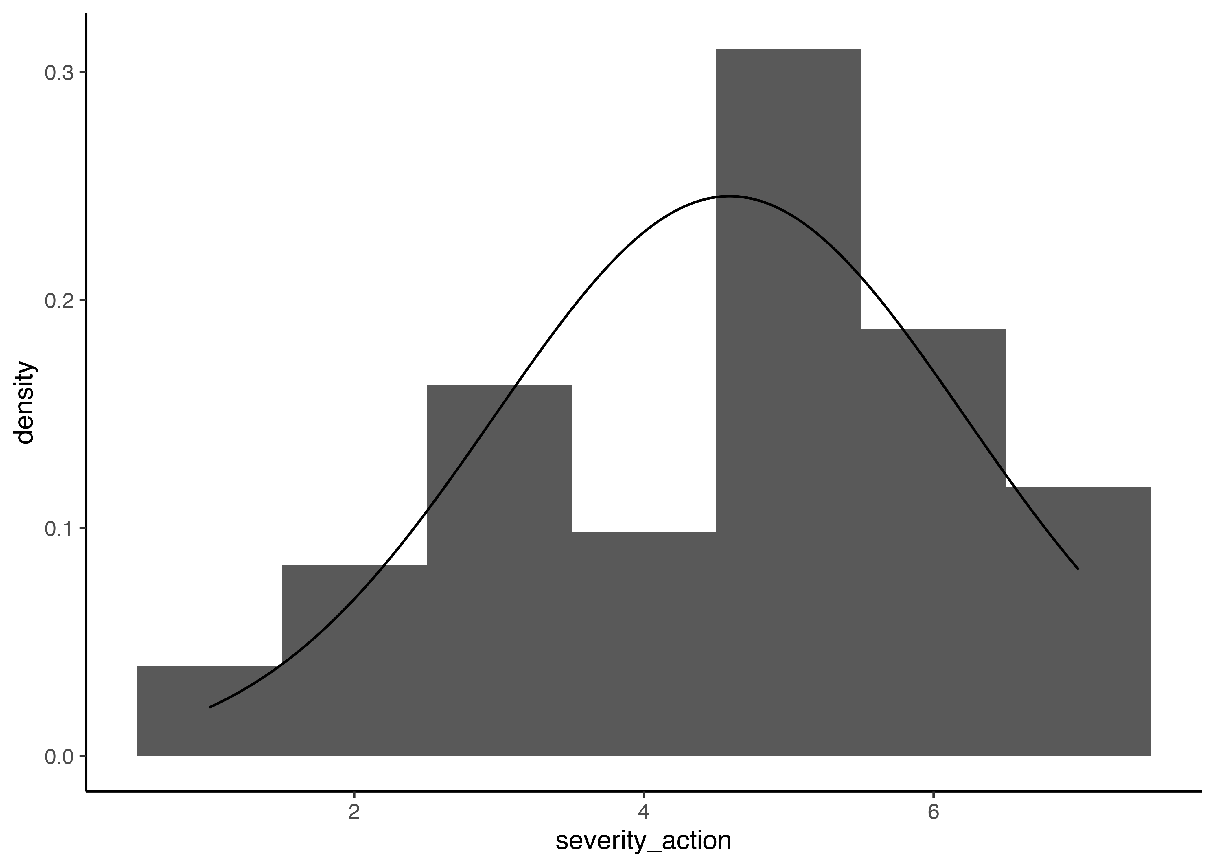
We get a mean of 4.59 and a sigma of 1.63. In the plot, you can see that even though the probability of getting ratings of 5 is higher than the probability of getting ratings of 4, that is not accounted for in the linear model.
Now, we are going to use an ordinal regression. In this case, we will use the function brm (Fit Bayesian generalized (non-)linear multivariate multilevel models) from the brms package.
1
2
3
4
5
6
m <- brm(severity_action ~ 1, data=memfor_data_s5, family=cumulative(link='probit'), cores=4)
summary(m)

intercept_draws <- m %>%
  gather_draws(b_Intercept[index]) %>%
  median_hdi
1
2
3
4
5
6
7
8
9
10
11
12
13
14
15
16
17
18
19
20
21
22
23
##  Family: cumulative
##   Links: mu = probit; disc = identity
## Formula: severity_action ~ 1
##    Data: memfor_data_s5 (Number of observations: 203)
##   Draws: 4 chains, each with iter = 2000; warmup = 1000; thin = 1;
##          total post-warmup draws = 4000
##
## Population-Level Effects:
##              Estimate Est.Error l-95% CI u-95% CI Rhat Bulk_ESS Tail_ESS
## Intercept[1]    -1.78      0.16    -2.11    -1.48 1.00     2980     2365
## Intercept[2]    -1.17      0.11    -1.40    -0.96 1.00     4489     3665
## Intercept[3]    -0.57      0.09    -0.76    -0.39 1.00     4486     3440
## Intercept[4]    -0.29      0.09    -0.46    -0.11 1.00     4305     3356
## Intercept[5]     0.52      0.09     0.34     0.70 1.00     4185     3308
## Intercept[6]     1.20      0.11     0.97     1.42 1.00     4900     3433
##
## Family Specific Parameters:
##      Estimate Est.Error l-95% CI u-95% CI Rhat Bulk_ESS Tail_ESS
## disc     1.00      0.00     1.00     1.00   NA       NA       NA
##
## Draws were sampled using sampling(NUTS). For each parameter, Bulk_ESS
## and Tail_ESS are effective sample size measures, and Rhat is the potential
## scale reduction factor on split chains (at convergence, Rhat = 1).
Notice that in this case, we have six thresholds that result in the 7 points of the Likert scale. The model gives and estimate of the value of the threshold and also confidence intervals that account for the uncertainty. Cool!
When we plot this, we are able to see the six thresholds with the values that were modeled from our data. You can see that the distance between the thresholds varies (as opposed to what we would assume when using a linear model). In this particular case, the distance between the thresholds are not very different, but we can see a shorter distance between the third (-0.57) and the fourth threshold (-0.29).
1
2
3
4
5
ggplot(intercept_draws, aes(x=.value)) +
  geom_line(aes(y=y), data=tibble(.value=seq(-3, 3, .01)) %>% mutate(y=dnorm(.value))) +
  geom_vline(aes(xintercept=.value)) +
  xlim(-3, 3) +
  theme_classic()
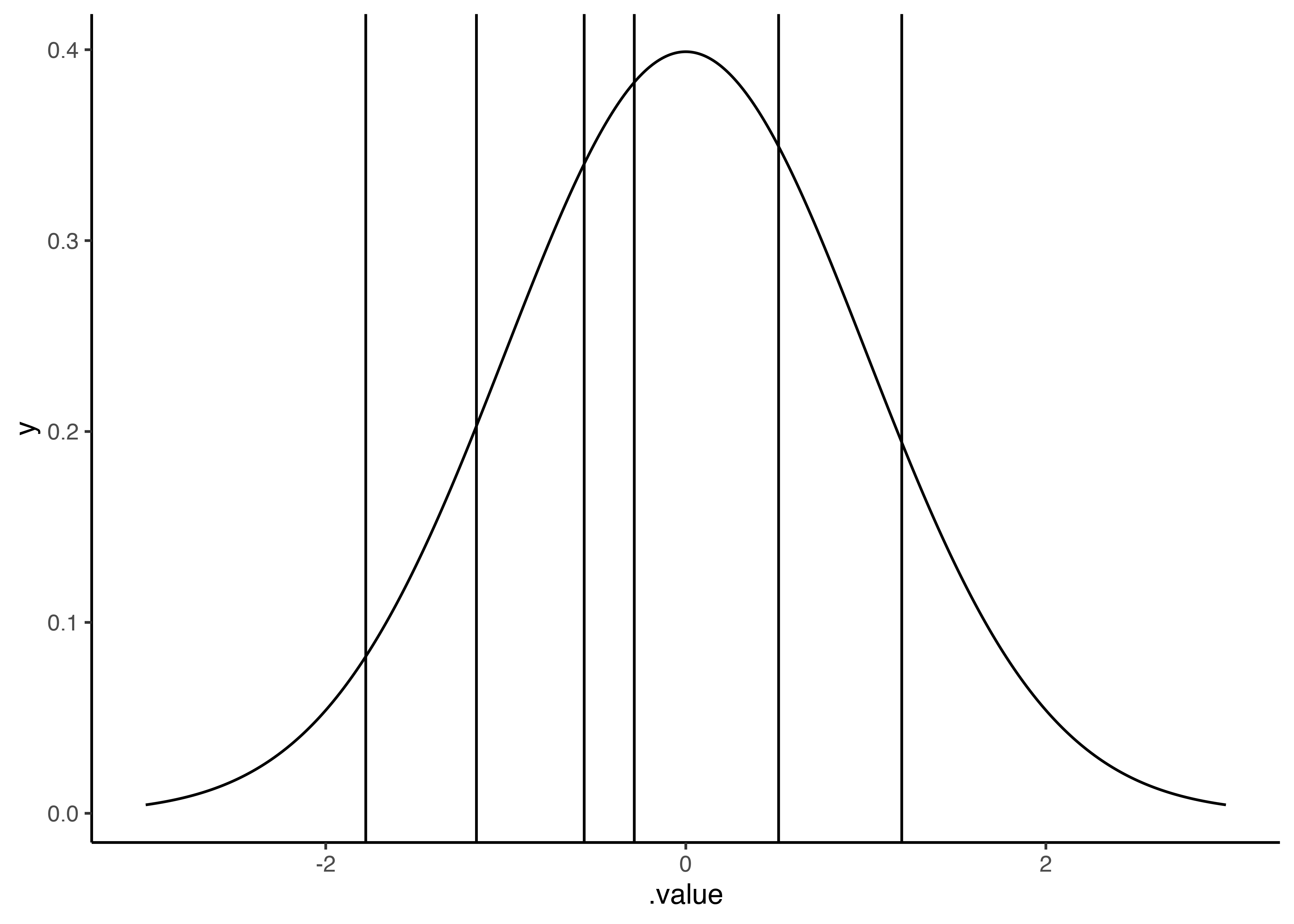
This just means that the probability of falling between different thresholds varies. In our case, it seems as if the probability of falling between the third and fourth threshold is lower than the probability of falling between the fourth and fifth threshold. This makes sense if we look back to the histogram of the linear regression that shows the probability of ratings of 5 (corresponds to the fourth and fifth threshold) seems to be higher that the probability of ratings of 4 (corresponds to the third and fourth threshold).
So now, let’s find those probabilities! For this, we have to create some data to estimate. In this case, since we have no predictors, we’ll just say X=1.
1
2
3
4
probabilities <- m %>%
  epred_draws(newdata=tibble(X=1)) %>%
  group_by(.draw) %>%
  mutate(.category=as.numeric(.category))
Now, lets plot our new ordinal model and see how it looks!
1
2
3
4
5
6
7
ggplot(memfor_data_s5, aes(x=severity_action)) +
  geom_histogram(aes(y=stat(density)), color='black', fill=NA, binwidth=1) +
  stat_ccdfinterval(aes(x=.category, y=.epred,
                    slab_alpha = stat(f)), thickness = 1,
                    show.legend=FALSE, data=probabilities) +
  ylab('Probability') + xlab('Severity of Action') +
  theme_classic()
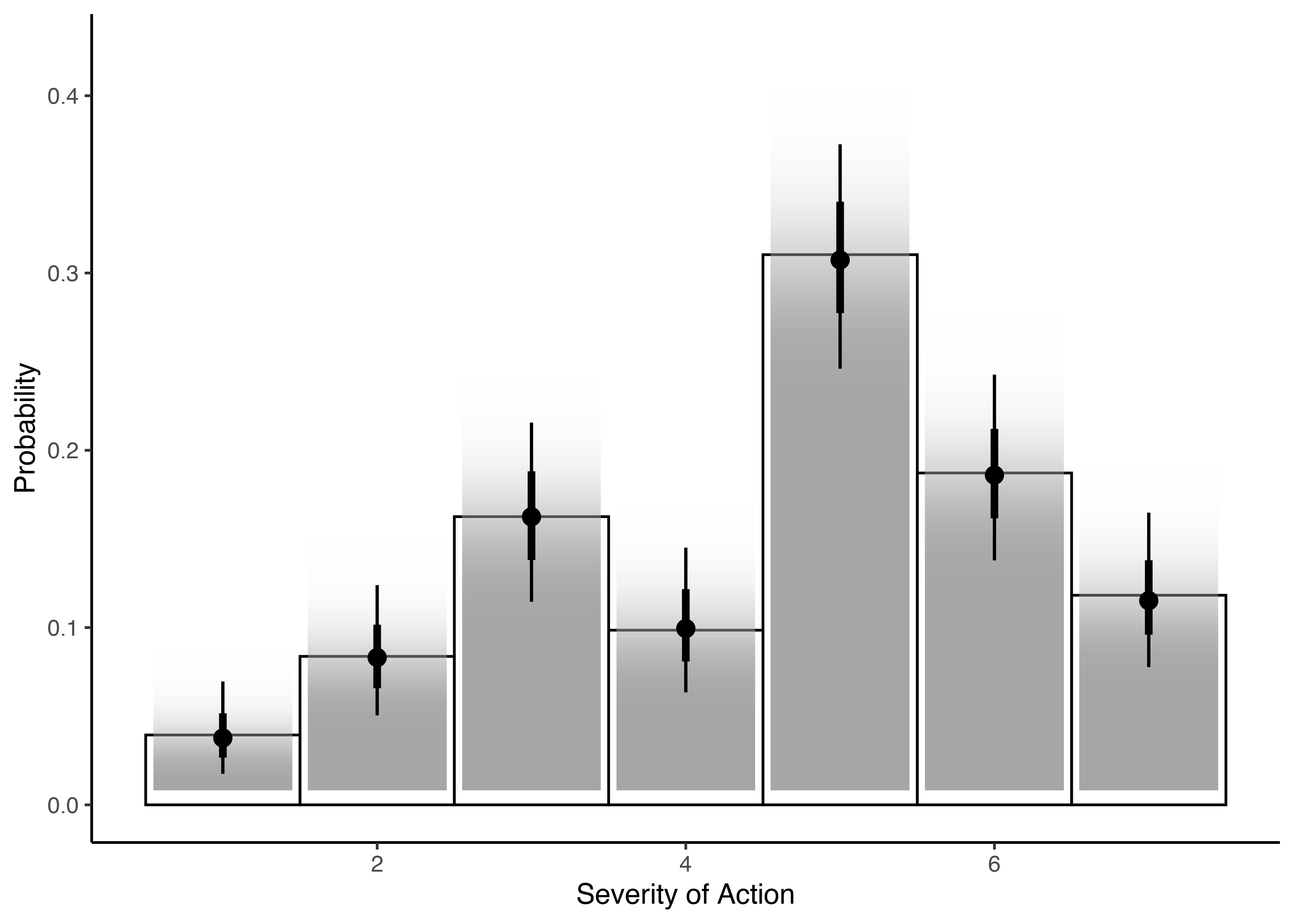
In this plot, you will see the data and the model, the probability for each point and, more interestingly, that the model accounts for the uncertainty and gives us confidence intervals. Nice!
But well, the idea would be to get to a point in which we find something that corresponds to the mean for a continuous variable. And to get that, what we need to do is to sum up the product of the probabilities by the category to which they belong.
1
2
3
4
5
draws_mean <- probabilities %>%
  summarize(mean=sum(.category * .epred))

draws_mean %>%
  median_hdi(mean)
1
2
3
4
## # A tibble: 1 × 6
##    mean .lower .upper .width .point .interval
##   <dbl>  <dbl>  <dbl>  <dbl> <chr>  <chr>
## 1  4.59   4.36   4.80   0.95 median hdi
And there you go! We have a ‘mean’ resulting from the ordinal regression that is useful for our research purposes. However, you could have noticed that the mean that we got with the ordinal regression (4.59) is exactly the same that we found when we did the good old linear regression. So, why should we get through all the trouble? Well, apparently this is not always the case always, and sometimes the values that you find differ, particularly when the thresholds are less equidistant. In those cases, the ordinal regression is the way to go since it actually accounts for this.
So, in our previous example we actually didn’t have predictors that could account for the distribution of our data. Now, lets try to model the same data, but with predictors.
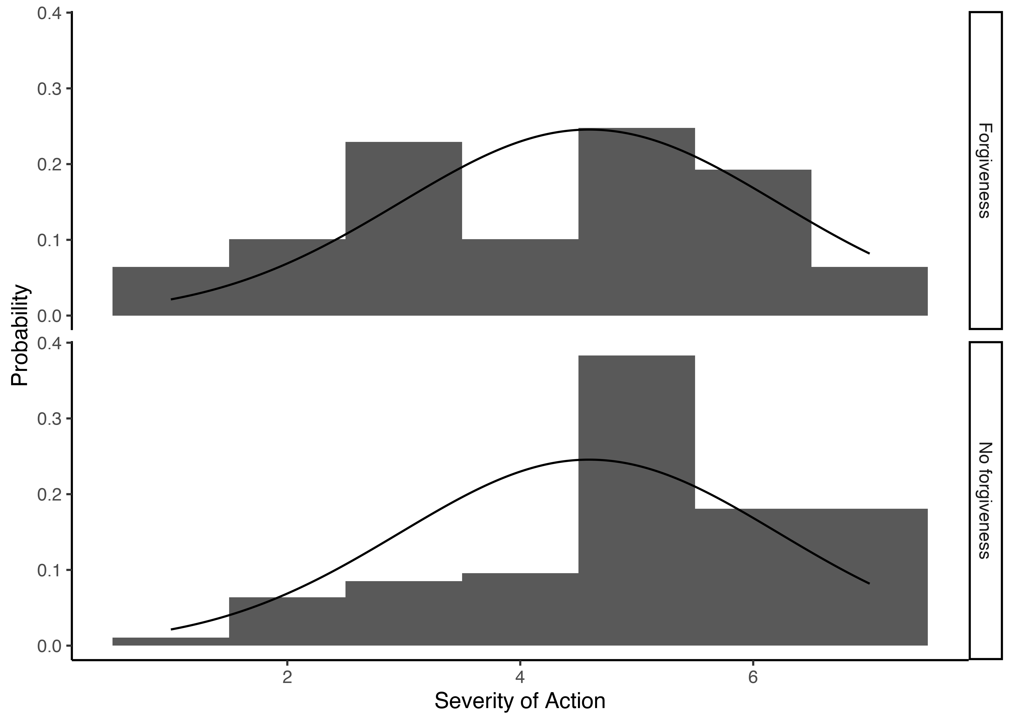
This data is part of my research on memory and forgiveness. For this study we asked participants to rate the severity of the harm committed by another person, and if the have or have not forgiven the wrongdoer. We would expect participants who didn’t forgive the wrongdoers to have higher ratings for the severity of the wrongdoing. Let’s see if that was the case.
First, lets see again how the gaussian model would look like:
1
2
3
4
5
6
7
8
9
10
11
m.gaussian_for <- brm(severity_action ~ condition, data=memfor_data_s5)
summary(m.gaussian)

ggplot(memfor_data_s5, aes(x=severity_action)) +
  geom_histogram(aes(y=stat(density)), binwidth=1) +
  geom_line(aes(x=.value, y=y), data=tibble(.value=seq(1, 7, .01)) %>%
              mutate(y=dnorm(.value, mean=mean(memfor_data_s5$severity_action),
                             sd=sd(memfor_data_s5$severity_action)))) +
  ylab('Probability') + xlab('Severity of Action') +
  facet_grid(condition ~ .) +
  theme_classic()
1
2
3
4
5
6
7
8
9
10
11
12
13
14
15
16
17
18
19
20
21
22
23
24
25
26
27
28
29
30
31
32
33
34
35
36
37
38
39
40
41
42
43
44
45
46
47
48
49
50
51
52
53
54
55
56
57
58
59
60
61
62
63
64
65
66
67
68
69
70
71
72
73
74
75
76
77
78
79
80
81
82
83
84
85
86
87
88
89
90
91
92
93
94
95
96
97
98
99
100
101
102
103
104
105
106
107
108
109
110
111
112
113
114
115
116
117
118
##
## SAMPLING FOR MODEL 'dbea789171f401b225cb6630884369c1' NOW (CHAIN 1).
## Chain 1:
## Chain 1: Gradient evaluation took 9e-06 seconds
## Chain 1: 1000 transitions using 10 leapfrog steps per transition would take 0.09 seconds.
## Chain 1: Adjust your expectations accordingly!
## Chain 1:
## Chain 1:
## Chain 1: Iteration:    1 / 2000 [  0%]  (Warmup)
## Chain 1: Iteration:  200 / 2000 [ 10%]  (Warmup)
## Chain 1: Iteration:  400 / 2000 [ 20%]  (Warmup)
## Chain 1: Iteration:  600 / 2000 [ 30%]  (Warmup)
## Chain 1: Iteration:  800 / 2000 [ 40%]  (Warmup)
## Chain 1: Iteration: 1000 / 2000 [ 50%]  (Warmup)
## Chain 1: Iteration: 1001 / 2000 [ 50%]  (Sampling)
## Chain 1: Iteration: 1200 / 2000 [ 60%]  (Sampling)
## Chain 1: Iteration: 1400 / 2000 [ 70%]  (Sampling)
## Chain 1: Iteration: 1600 / 2000 [ 80%]  (Sampling)
## Chain 1: Iteration: 1800 / 2000 [ 90%]  (Sampling)
## Chain 1: Iteration: 2000 / 2000 [100%]  (Sampling)
## Chain 1:
## Chain 1:  Elapsed Time: 0.008773 seconds (Warm-up)
## Chain 1:                0.009006 seconds (Sampling)
## Chain 1:                0.017779 seconds (Total)
## Chain 1:
##
## SAMPLING FOR MODEL 'dbea789171f401b225cb6630884369c1' NOW (CHAIN 2).
## Chain 2:
## Chain 2: Gradient evaluation took 1e-06 seconds
## Chain 2: 1000 transitions using 10 leapfrog steps per transition would take 0.01 seconds.
## Chain 2: Adjust your expectations accordingly!
## Chain 2:
## Chain 2:
## Chain 2: Iteration:    1 / 2000 [  0%]  (Warmup)
## Chain 2: Iteration:  200 / 2000 [ 10%]  (Warmup)
## Chain 2: Iteration:  400 / 2000 [ 20%]  (Warmup)
## Chain 2: Iteration:  600 / 2000 [ 30%]  (Warmup)
## Chain 2: Iteration:  800 / 2000 [ 40%]  (Warmup)
## Chain 2: Iteration: 1000 / 2000 [ 50%]  (Warmup)
## Chain 2: Iteration: 1001 / 2000 [ 50%]  (Sampling)
## Chain 2: Iteration: 1200 / 2000 [ 60%]  (Sampling)
## Chain 2: Iteration: 1400 / 2000 [ 70%]  (Sampling)
## Chain 2: Iteration: 1600 / 2000 [ 80%]  (Sampling)
## Chain 2: Iteration: 1800 / 2000 [ 90%]  (Sampling)
## Chain 2: Iteration: 2000 / 2000 [100%]  (Sampling)
## Chain 2:
## Chain 2:  Elapsed Time: 0.009016 seconds (Warm-up)
## Chain 2:                0.008926 seconds (Sampling)
## Chain 2:                0.017942 seconds (Total)
## Chain 2:
##
## SAMPLING FOR MODEL 'dbea789171f401b225cb6630884369c1' NOW (CHAIN 3).
## Chain 3:
## Chain 3: Gradient evaluation took 2e-06 seconds
## Chain 3: 1000 transitions using 10 leapfrog steps per transition would take 0.02 seconds.
## Chain 3: Adjust your expectations accordingly!
## Chain 3:
## Chain 3:
## Chain 3: Iteration:    1 / 2000 [  0%]  (Warmup)
## Chain 3: Iteration:  200 / 2000 [ 10%]  (Warmup)
## Chain 3: Iteration:  400 / 2000 [ 20%]  (Warmup)
## Chain 3: Iteration:  600 / 2000 [ 30%]  (Warmup)
## Chain 3: Iteration:  800 / 2000 [ 40%]  (Warmup)
## Chain 3: Iteration: 1000 / 2000 [ 50%]  (Warmup)
## Chain 3: Iteration: 1001 / 2000 [ 50%]  (Sampling)
## Chain 3: Iteration: 1200 / 2000 [ 60%]  (Sampling)
## Chain 3: Iteration: 1400 / 2000 [ 70%]  (Sampling)
## Chain 3: Iteration: 1600 / 2000 [ 80%]  (Sampling)
## Chain 3: Iteration: 1800 / 2000 [ 90%]  (Sampling)
## Chain 3: Iteration: 2000 / 2000 [100%]  (Sampling)
## Chain 3:
## Chain 3:  Elapsed Time: 0.008609 seconds (Warm-up)
## Chain 3:                0.00889 seconds (Sampling)
## Chain 3:                0.017499 seconds (Total)
## Chain 3:
##
## SAMPLING FOR MODEL 'dbea789171f401b225cb6630884369c1' NOW (CHAIN 4).
## Chain 4:
## Chain 4: Gradient evaluation took 3e-06 seconds
## Chain 4: 1000 transitions using 10 leapfrog steps per transition would take 0.03 seconds.
## Chain 4: Adjust your expectations accordingly!
## Chain 4:
## Chain 4:
## Chain 4: Iteration:    1 / 2000 [  0%]  (Warmup)
## Chain 4: Iteration:  200 / 2000 [ 10%]  (Warmup)
## Chain 4: Iteration:  400 / 2000 [ 20%]  (Warmup)
## Chain 4: Iteration:  600 / 2000 [ 30%]  (Warmup)
## Chain 4: Iteration:  800 / 2000 [ 40%]  (Warmup)
## Chain 4: Iteration: 1000 / 2000 [ 50%]  (Warmup)
## Chain 4: Iteration: 1001 / 2000 [ 50%]  (Sampling)
## Chain 4: Iteration: 1200 / 2000 [ 60%]  (Sampling)
## Chain 4: Iteration: 1400 / 2000 [ 70%]  (Sampling)
## Chain 4: Iteration: 1600 / 2000 [ 80%]  (Sampling)
## Chain 4: Iteration: 1800 / 2000 [ 90%]  (Sampling)
## Chain 4: Iteration: 2000 / 2000 [100%]  (Sampling)
## Chain 4:
## Chain 4:  Elapsed Time: 0.00879 seconds (Warm-up)
## Chain 4:                0.009456 seconds (Sampling)
## Chain 4:                0.018246 seconds (Total)
## Chain 4:
##  Family: gaussian
##   Links: mu = identity; sigma = identity
## Formula: severity_action ~ 1
##    Data: memfor_data_s5 (Number of observations: 203)
##   Draws: 4 chains, each with iter = 2000; warmup = 1000; thin = 1;
##          total post-warmup draws = 4000
##
## Population-Level Effects:
##           Estimate Est.Error l-95% CI u-95% CI Rhat Bulk_ESS Tail_ESS
## Intercept     4.59      0.12     4.37     4.81 1.00     3418     2836
##
## Family Specific Parameters:
##       Estimate Est.Error l-95% CI u-95% CI Rhat Bulk_ESS Tail_ESS
## sigma     1.63      0.08     1.48     1.81 1.00     3104     2644
##
## Draws were sampled using sampling(NUTS). For each parameter, Bulk_ESS
## and Tail_ESS are effective sample size measures, and Rhat is the potential
## scale reduction factor on split chains (at convergence, Rhat = 1).
Now, let’s try with the ordinal regression
1
2
3
4
5
6
m_for <- brm(severity_action ~ condition, data=memfor_data_s5, family=cumulative(link='probit'), cores=4)
summary(m_for)

intercept_draws <- m_for %>%
  gather_draws(b_Intercept[index]) %>%
  median_hdi
1
2
3
4
5
6
7
8
9
10
11
12
13
14
15
16
17
18
19
20
21
22
23
24
25
26
27
28
29
30
31
32
##  Family: cumulative
##   Links: mu = probit; disc = identity
## Formula: severity_action ~ condition
##    Data: memfor_data_s5 (Number of observations: 203)
##   Draws: 4 chains, each with iter = 2000; warmup = 1000; thin = 1;
##          total post-warmup draws = 4000
##
## Population-Level Effects:
##                        Estimate Est.Error l-95% CI u-95% CI Rhat Bulk_ESS
## Intercept[1]              -1.60      0.17    -1.94    -1.28 1.00     3958
## Intercept[2]              -0.96      0.13    -1.21    -0.71 1.00     4993
## Intercept[3]              -0.34      0.12    -0.56    -0.11 1.00     4855
## Intercept[4]              -0.04      0.11    -0.26     0.17 1.00     5094
## Intercept[5]               0.78      0.12     0.56     1.01 1.00     5167
## Intercept[6]               1.48      0.14     1.22     1.77 1.00     5477
## conditionNoforgiveness     0.54      0.15     0.25     0.84 1.00     5208
##                        Tail_ESS
## Intercept[1]               2918
## Intercept[2]               3093
## Intercept[3]               3470
## Intercept[4]               3392
## Intercept[5]               3526
## Intercept[6]               3030
## conditionNoforgiveness     2939
##
## Family Specific Parameters:
##      Estimate Est.Error l-95% CI u-95% CI Rhat Bulk_ESS Tail_ESS
## disc     1.00      0.00     1.00     1.00   NA       NA       NA
##
## Draws were sampled using sampling(NUTS). For each parameter, Bulk_ESS
## and Tail_ESS are effective sample size measures, and Rhat is the potential
## scale reduction factor on split chains (at convergence, Rhat = 1).
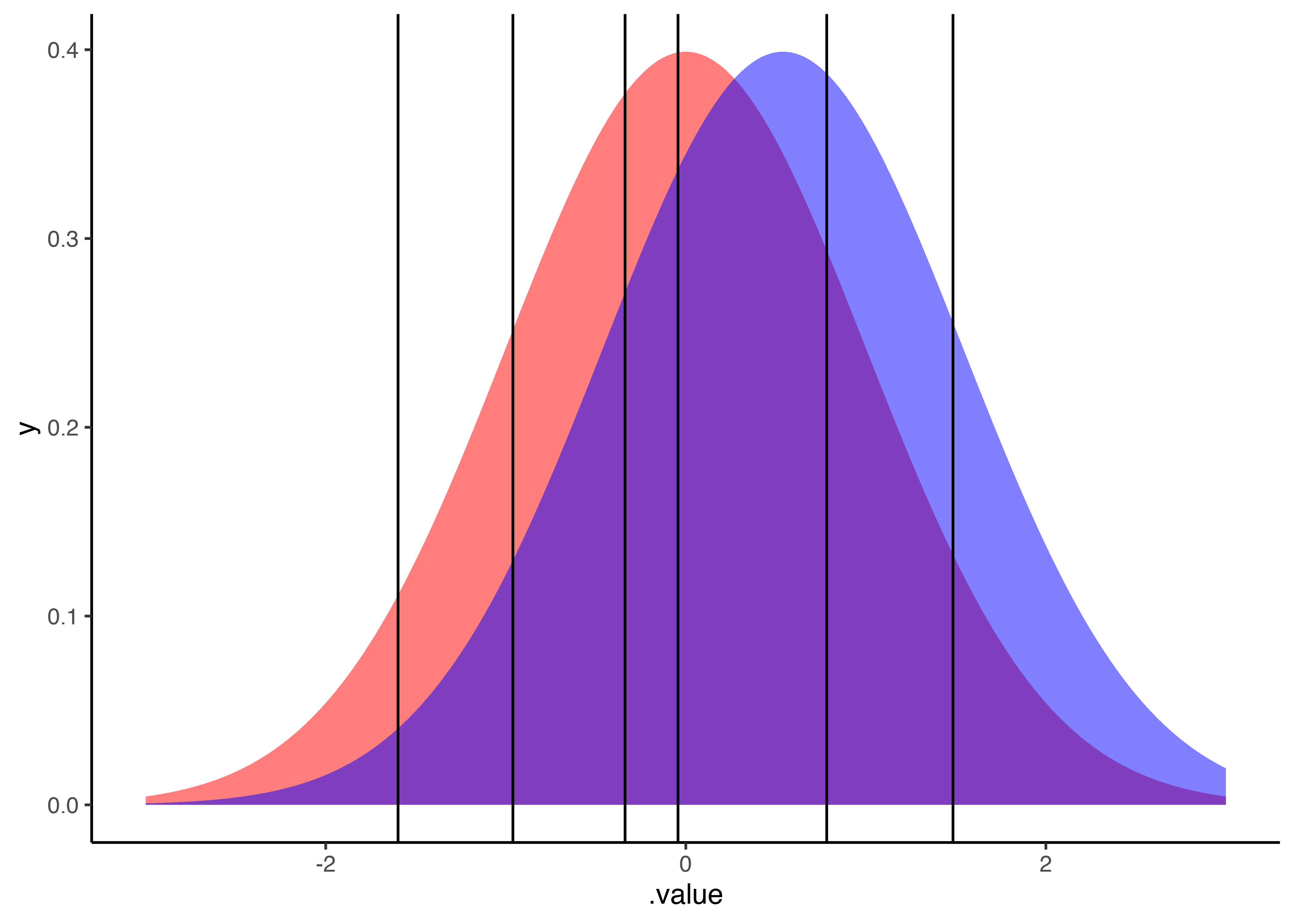
Now, let’s take a look at how the distribution looks when we include forgiveness as a condition
1
2
3
4
5
6
ggplot(intercept_draws, aes(x=.value)) +
  geom_area(aes(y=y), fill='red', alpha=.5, data=tibble(.value=seq(-3, 3, .01)) %>% mutate(y=dnorm(.value))) +
  geom_area(aes(y=y), fill='blue', alpha=.5, data=tibble(.value=seq(-3, 3, .01)) %>% mutate(y=dnorm(.value, mean=0.54))) +
  geom_vline(aes(xintercept=.value)) +
  xlim(-3, 3) +
  theme_classic()
Now let’s find the probabilities by condition
1
2
3
4
probabilities_for <- m_for %>%
  epred_draws(newdata=tibble(condition=unique(memfor_data_s5$condition))) %>%
  group_by(condition, .draw) %>%
  mutate(.category=as.numeric(.category))
And now, this is how our ordinal regression looks like:
1
2
3
4
5
6
7
8
ggplot(memfor_data_s5, aes(x=severity_action)) +
  geom_histogram(aes(y=stat(density)), color='black', fill=NA, binwidth=1) +
  stat_ccdfinterval(aes(x=.category, y=.epred,
                        slab_alpha = stat(f)), thickness = 1,
                    show.legend=FALSE, data=probabilities_for) +
  facet_grid(condition ~ .) +
  ylab('Probability') + xlab('Severity of Action') +
  theme_classic()
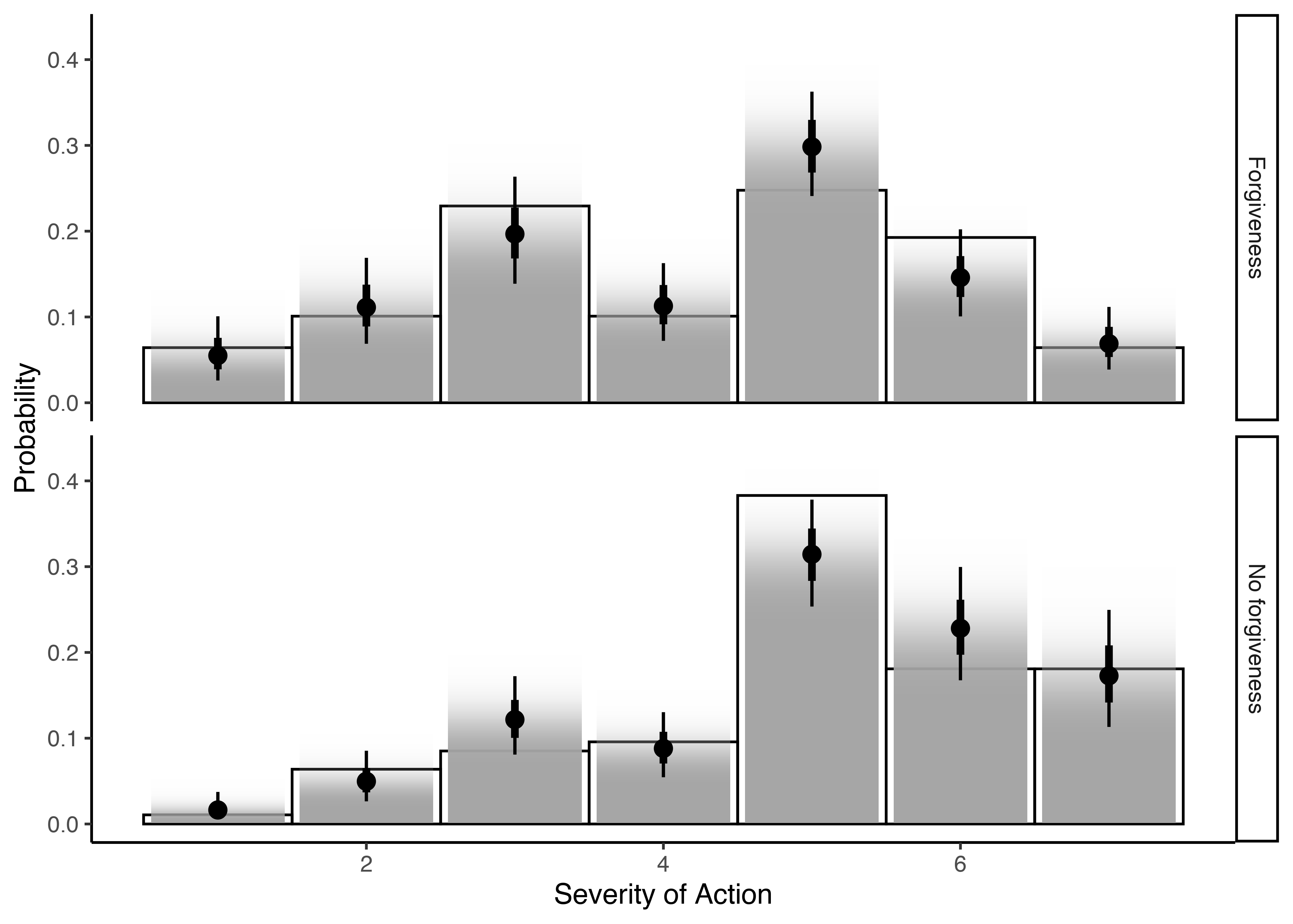
And here are our means by condition!
1
2
3
4
5
draws_mean_for <- probabilities_for %>%
  summarize(mean=sum(.category * .epred))

draws_mean_for %>%
  median_hdi(mean)
1
2
3
4
5
## # A tibble: 2 × 7
##   condition       mean .lower .upper .width .point .interval
##   <chr>          <dbl>  <dbl>  <dbl>  <dbl> <chr>  <chr>
## 1 Forgiveness     4.21   3.90   4.51   0.95 median hdi
## 2 No forgiveness  5.02   4.72   5.31   0.95 median hdi