Bayesian Indices of Significance
This week we talked about the recent paper Indices of Effect Existence and Significance in the Bayesian Framework by Dominique Makowski, Mattan S. Ben-Shachar, S. H. Annabel Chen, and Daniel Lüdecke, which is a fantastic reference for deciding how to test your hypotheses with Bayesian statistics. This post is a summary of the paper, which I definitely recommend to anyone venturing into Bayesian statistics.
If you already know what most of these things are and you want to know
how to compute them in R, check out the bayestestR
package,
spearheaded by the same team.
Overview
Introduction
In Frequentist statistics, we try to estimate a single parameter value that makes the data most likely (i.e., we look for a Maximum Likelihood Estimate). In this view, the data are random, but the effects are fixed in that we assume there is a single “correct” value that we’re looking for. To test hypotheses in this framework, researchers most often use Null Hypothesis Significance Testing (NHST), in which they calculate a p-value, and reject the null hypothesis if this value is small enough. NHST is widely used because it is easy to perform, controls for type 1 error rates, and supposedly gives you a clear-cut answer to your research question given the data. However, Frequentist NHST has four major problems: (a) it never allows you to accept the null hypothesis (you can only reject it), (b) it places emphasis on effect significance, not effect size, (c) it relies on an arbitrary threshold for significance, and as a result, (d) it is associated with problems like p-hacking, publication bias, and the replicability crisis.
To remedy some of these issues, many researchers are now moving to Bayesian statistics, where we estimate a full distribution of possible parameter values (i.e., a posterior) in contrast to just a single value. I won’t cover Bayesian statistics here, but check out this post for a refresher. One particular advantage of Bayesian statistics is that there are many ways of quantifying the size or importance of an effect, so we aren’t just stuck with p-values. But this blessing is also a curse: since we have so many different metrics of significance, there is little agreement about which metrics are best for which purposes, and this confusion can be a major hurdle for anyone trying to learn Bayesian statistics for themselves.
Methods
This paper is geared toward solving this problem: by testing a bunch of these metrics under a range of conditions, we can see what properties they have, and decide when to use them. In particular, the authors simulate linear and logistic regressions, calculate indices of significance, and compare them to each other.
Indices
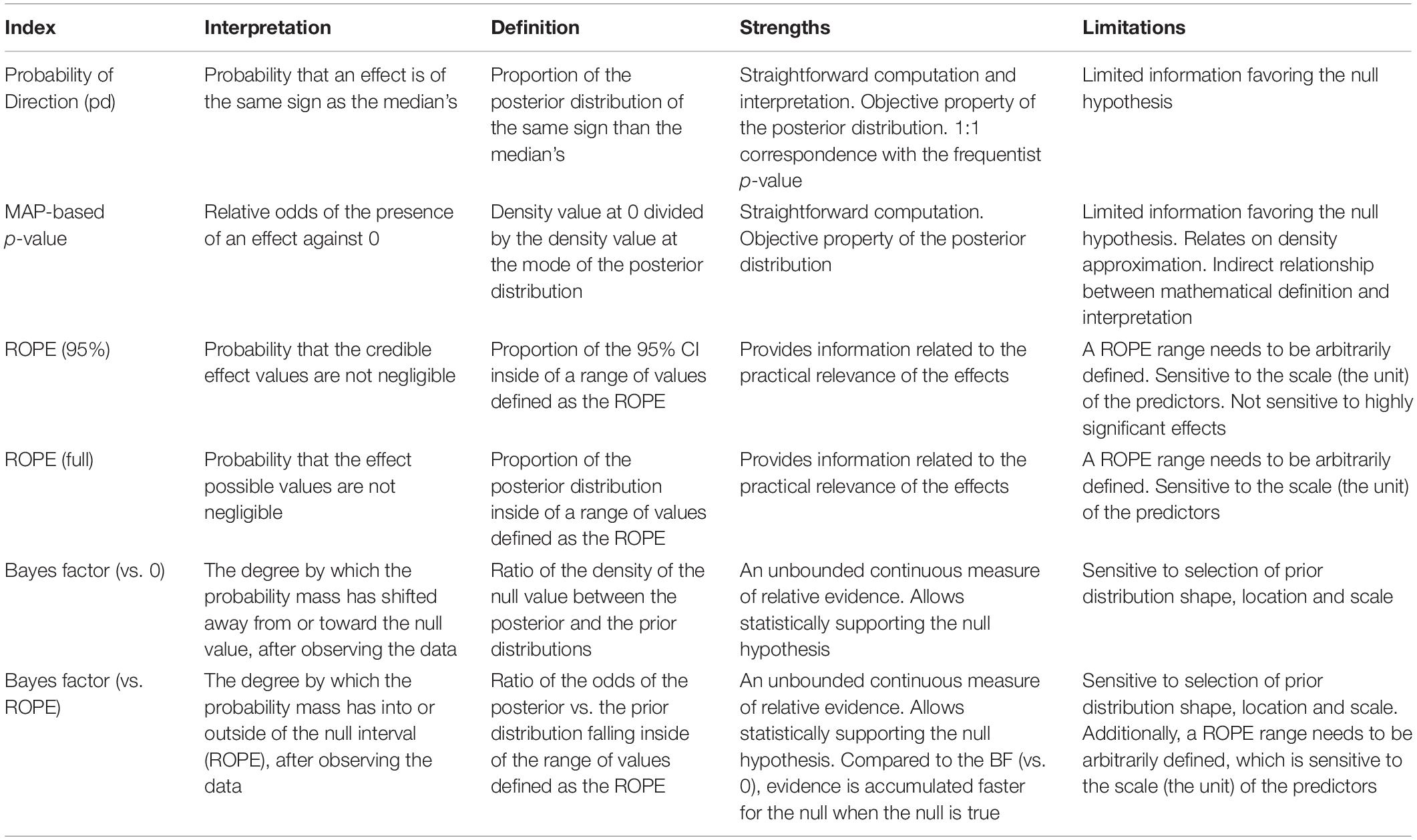
Before talking about the simulations themselves, let’s introduce the indices of significance that the authors tested, summarized in this figure:
Frequentist p-Value
As I mentioned before, the Frequentist p-value is what researchers typically use to test hypotheses in psychology and neuroscience. The p-value is the probability \(P(\lvert\theta\rvert \ge \lvert\hat{\theta}\rvert \; | \; \mathcal{H}_0, \mathcal{I})\) that we would observe an statistic \(\theta\) as big as the one we observed \(\hat{\theta}\), given that the null hypothesis \(\mathcal{H}_0\) is true and given our testing and stopping intentions \(\mathcal{I}\) (e.g., the intention to collect 50 data points and to run a single statistical test). There are a couple things to note here. First, since the p-value assumes the null hypothesis, it can not be interpreted as the probability that the null hypothesis is correct. So even if \(p = 1\), you cannot accept the null hypothesis. Second, since it assumes a set of testing and stopping intentions, you (as a researcher) are obligated to follow those intentions. So no optional stopping, p-hacking, or anything like that. Finally, p-values do not tell us anything about the size of an effect, only about our certainty that the effect exists.
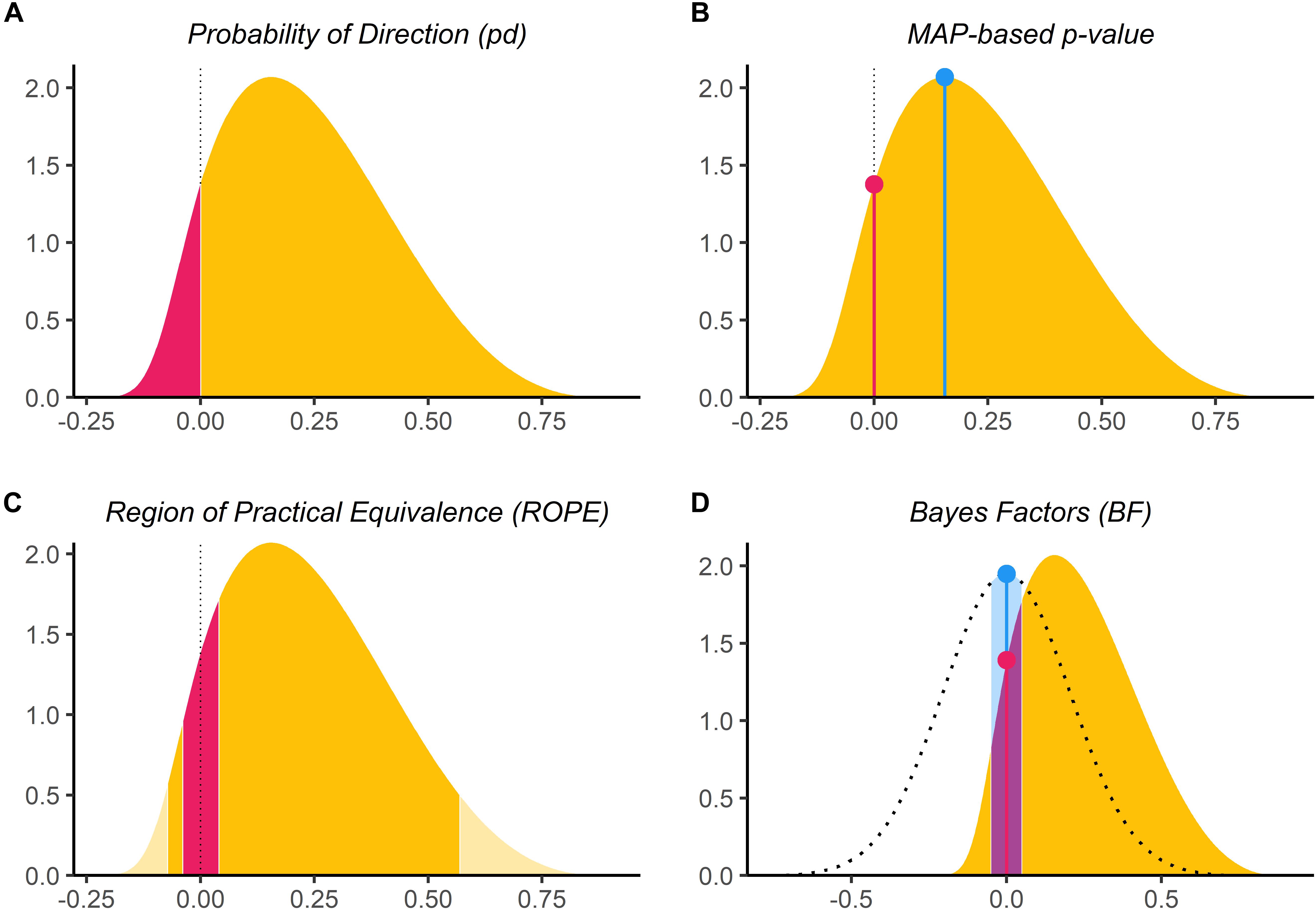
Probability of Direction (pd)
Probability of direction is a new Bayesian measure of significance that is probably the simplest one. pd is defined as the probability that a parameter is strictly positive \(P(\theta > 0 | X)\) or strictly negative \(P(\theta < 0 | X)\), whichever is more likely. In other words, it is the proportion of the posterior distribution that is positive if most of the posterior is positive, or as the proportion of the posterior distribution that is negative if most of the posterior is negative. It lies between 50% (where half of the posterior is positive and half is negative) and 100% (where all of the posterior is positive or all of it is negative).
MAP-based p-Value (p-MAP)
The MAP-based p-value is a Bayesian measure intended to resemble the Frequentist p-value, defined as the odds that the parameter has against the null hypothesis. It is the ratio \(P(\theta = 0) / P(\theta = MAP)\) of the posterior probability that the parameter equals 0 (or some other null value of interest) divided by the posterior probability that the parameter is equal to the maximum a posteriori (or most likely) value. Here a value of 0 means that the null hypothesis is impossible (i.e., the parameter cannot be 0) and a value of 1 means that the null hypothesis is most likely (i.e., the posterior mode is at 0).
Region of Practical Equivalence (ROPE)
The Region of Practical Equivalence assumes that there is a range of parameter values (called the ROPE) that are so small, they might as well be considered as practically equivalent to zero. To define this range, it is common to use a standardized effect size of [-.1, .1], which is usually considered a negligible effect size. Once we have the ROPE, we can simply check how much of the posterior lies within that range: ROPE (full) = \(P(-ROPE \le \theta \le ROPE)\). When this probability is 0, we can say that the effect is significant (since the parameter lies entirely outside of the null region). When it is 1, we can say that the parameter is practically equivalent to 0 (since all of the posterior lies inside the null region).
Some argue that this over-weights parameter values that are extremely unlikely, and so we should exclude them from this proportion. To do so, we simply condition that the parameter lies within some highest density interval (HDI), such as the 95% HDI: ROPE (HDI) = \(P(-ROPE \le \theta \le ROPE \; | \; lowerHDI \le \theta \le upperHDI)\). Both versions are essentially the same, but ROPE (full) considers the entire posterior, whereas ROPE (HDI) considers only the most probable values. This has the effect of making the ROPE values more robust at the cost of being less sensitive, where choosing an HDI close to 100% prefers sensitivity and choosing smaller HDIs favors robustness.
Bayes Factor (BF)
For better or for worse, the Bayes Factor is probably the most well-known and most widely-used Bayesian metrics of significance. Bayes’ rule tells us that to get the posterior probability \(P(\mathcal{H} \; | \; \mathcal{D})\) of a hypothesis \(\mathcal{H}\) given the data \(\mathcal{D}\), we need to start with a prior probability \(P(\mathcal{H})\), and multiply by the likelihood of the data given the hypothesis, normalized by the probability of the data:
When we want to compare two hypotheses \(\mathcal{H}_0\) and \(\mathcal{H}_a\), we can just take the ratio of their posterior probabilities, known as the posterior odds (note that the \(P(\mathcal{D})\)s cancel out):
So the posterior odds break apart into the BF, which is just the likeliihood ratio, and the prior odds, which specify the extent to which we initially trust \(\mathcal{H}_0\) over \(\mathcal{H}_a\). Usually we don’t prefer one hypothesis over the other a priori, so this ratio is just 1, and the posterior odds are just the BF.
Just like how there are two versions of the ROPE, there are also two possible versions of the BF for testing against a null hypothesis. When the null hypothesis is that \(\theta = 0\) (i.e., a point-null), the BF tells us whether our belief that \(\theta = 0\) has increased (BF > 1) or decreased (BF < 1). But we can also choose a null hypothesis that \(-ROPE \le \theta \le ROPE\), where \(ROPE\) is some small value we consider to be practically equivalent to zero. Then the BF tells us whether our belief that \(\theta\) lies in this range has increased or decreased after seeing the data.
Simulation
Now that we know what each of the measures are, how do we compare them? Easy: we simulate some data, and calculate them! In this case, the authors simulated data for linear and logistic regression with a pre-defined ground-truth presence or absence of an effect, a pre-defined sample size, and a pre-defined noise level. Varying each of these factors, they made 36,000 datasets in total, and calculated each of the above metrics over the corresponding linear/logistic regression.
Results
To compare each of the measures, the authors looked at the impact of sample size on each measure, the impact of noise, the relationship with the Frequentist p-value, and the relationship between the measures.
Impact of Sample Size
As you can see below, the measures exhibit two overall patterns.
The Frequentist p-value, pd, and p-MAP all indicate increasing significance with increasing sample size when there truly is an effect to be detected. However, when the null hypothesis is true, these measures show no relationship with sample size.
On the other hand, both the ROPE and the BF seem to be influenced by sample size regardless of whether the null hypothesis is true or false. When the \(\mathcal{H}_0\) is true, they show a higher preference for the null over the alternate hypothesis with larger samples. In contrast, when the null is false, they show a greater preference for the alternative hypothesis with larger samples. There also doesn’t seem to be a big difference between the two ROPEs or between the two BFs.

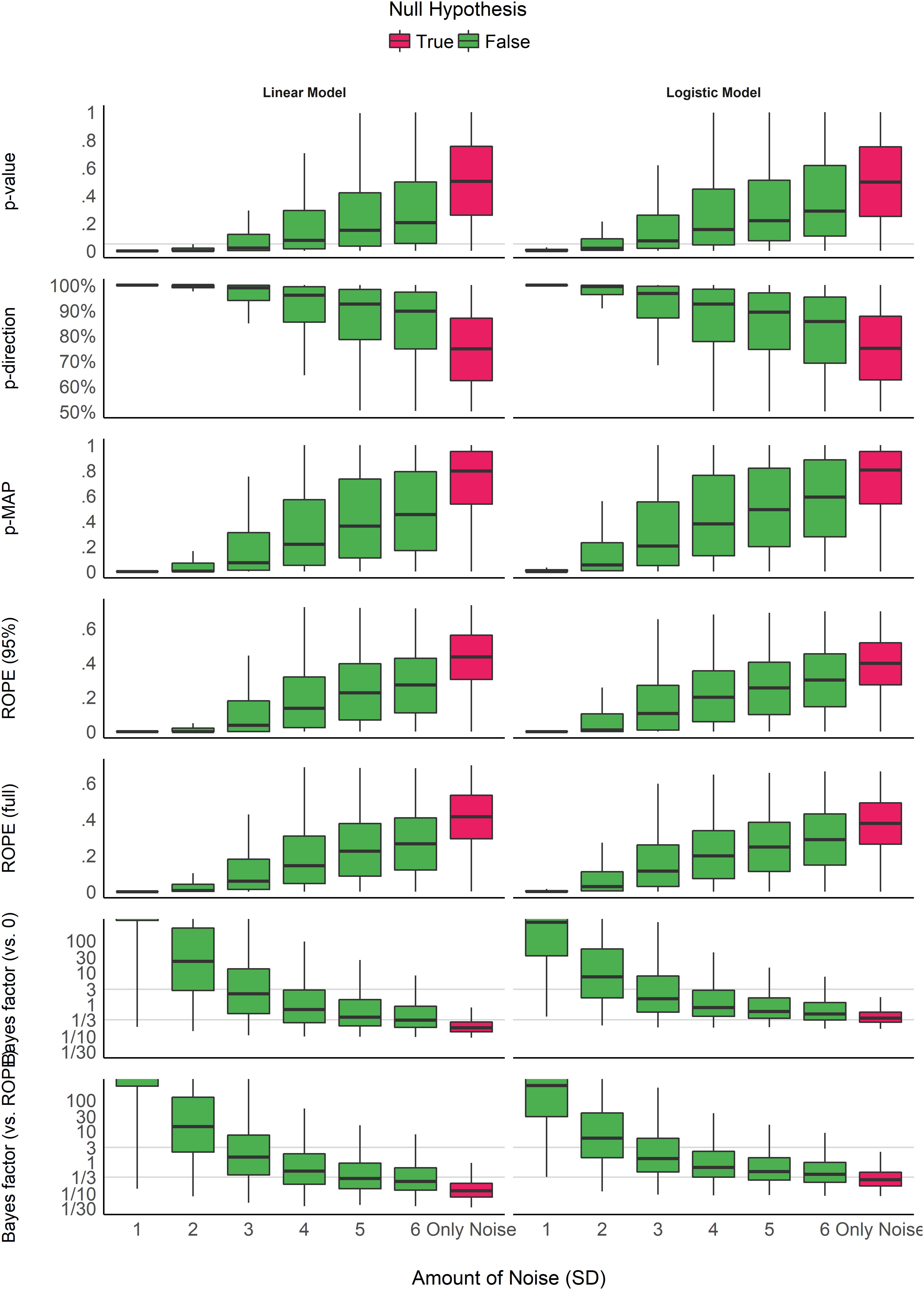
Impact of Noise
Unlike the impact of sample size, all of the measures seem to be similarly impacted by noise in the predictor variable- the more noise, the less “significant” of a result. However, while most of the measures seem to have more variability in the presence of noise, the BF has less variability with increasing noise (indicating a convergence on the null hypothesis).
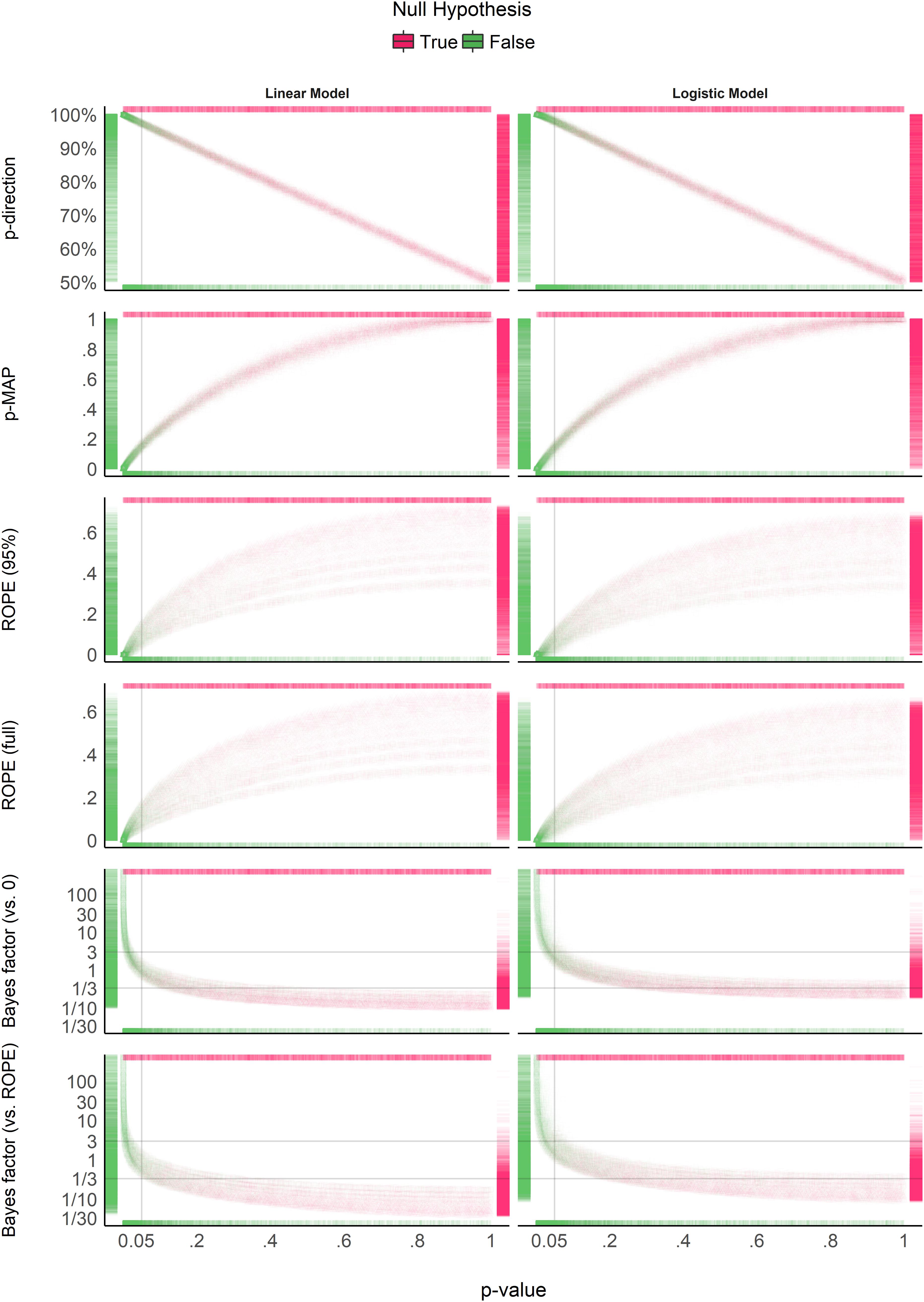
Relationship with p-value
As you can probably tell at this point, pd and p-MAP are strongly related to the Frequentist p-value, whereas the ROPE and BF are not trivially related to the p-value. While p-MAP has a curvilinear relationship to the p-value, pd is approximately linearly related through the following formula: \(p_{two-tailed} = 2(1 - pd)\). This implies that pd is probably a nice thing to report to the pesky reviewer demanding p-values.
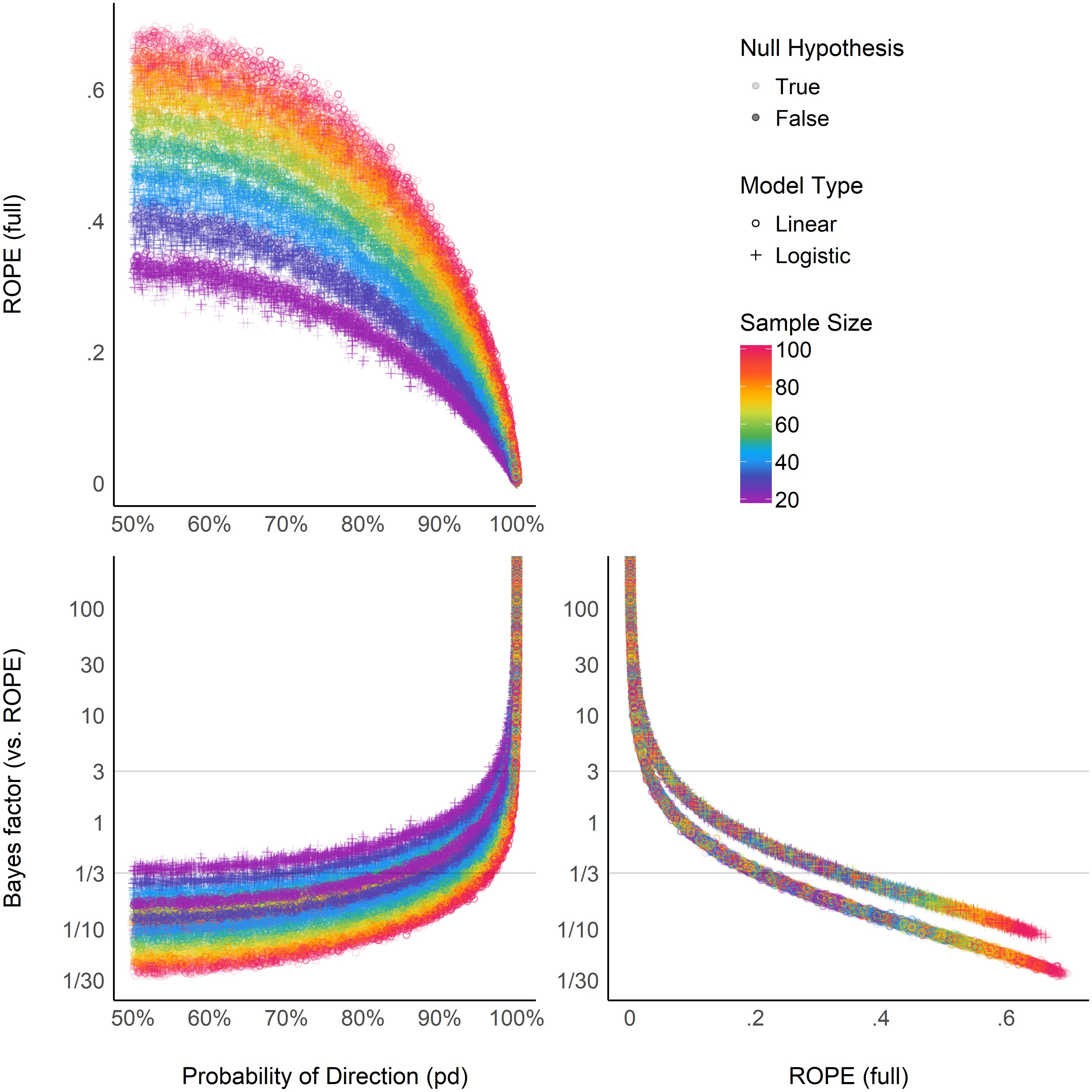
Relationship Between ROPE (full), pd, and BF (vs. ROPE)
Finally, the authors investigated the relationships between the BF, the ROPE, and pd (which as we saw directly corresponds to p-values). The left two plots show that both the BF and the ROPE are related to pd, but these relationships are modulated by sample size. On the right, we can see that the BF and ROPE measures are directly related, but that this relationship depends on the type of the model being tested (linear or logistic).
Discussion
Overall, the authors concluded that it seems like these measures break down into two families, which each indicate separate things.
-
The p-value, pd, and p-MAP all seem to indicate the existence of an effect. When a true effect exists, they are related to sample size, but when no effect exists, they don’t carry any information at all. So these measures can be interpreted as one’s certainty that an effect exists (or not).
-
The BF and the ROPE, on the other hand, seem to truly indicate the significance of an effect in the common sense of the word (i.e., effect size or importance). These two measures care about both the presence and the absence of an effect.
Because of this division, the authors recommend adopting an existence-significance framework in which you interpret the measures accordingly.
Reporting Guidelines
The tldr version of this post is that some measures (p, pd, and p-MAP) indicate the existence of an effect and others (BF, ROPE) the significance. So, it’s best to report (at least) one measure from each category. In terms of existence, pd is probably the best measure to report because it’s easy to interpret and because it directly corresponds to the well-known but misunderstood p-value. To report significance, the authors recommend using BF (vs ROPE) when you have informative priors (since the BF is influenced by prior information), and to use the ROPE (full) when you don’t (since the ROPE is pretty much constant under any not-super-informative prior). Of course none of these measures are perfect or good for everything, so you consult the table below for a nice summary.
I found this paper to be incredibly useful in reporting my own analyses and interpreting my results. If you’re relatively new to Bayesian stats, hopefully this encouraged you to try it out!