Drift Diffusion Models for Psychological Science

Intro To Computational Modeling

As scientists we collect all sorts of data. Decision data (which fruits to people prefer?), neural data (which neurons fire when looking at fruits?), reaction time data (how quickly do people identify fruit from non-fruits?), etc. Computational modeling in psychology is all about gaining insights about the brain and behavior from this data by designing mathematical formulations that produce fake data that looks similar to that produced by humans (or animals or whatever we are modeling). The closer and more reliably we can reproduce human-like data with our math equations, the better our model is, and the closer we get to maybe gaining some insights into the computations for the brain.

As an example, early modelers of reward learning (think Pavlov’s dog) came up with a mathematical formulation called the prediction error, which was simply the difference between expected reward and the actual reward received from an action (Vt - Rt, where V is the expected reward on trial t). Later, it was shown that this hypothetical construct maps almost perfectly onto the firing rate of dopamine neurons in the midbrain. This gave massive support to the idea that prediction errors are a fundamental calculation in the brain during reward learning.

Hopefully you see just how useful computational modeling can be. As I said, modeling is about writing math equations that produce fake data that looks as similar to real data as possible. Once we have developed really good models, we can next perform model fitting (also called parameter estimation) to find the particular model parameters that would make the real data the most likely if the model was the one producing it instead. You’ll often hear the term maximumum likelihood estimation or MLE used by modelers. All that is a bit outside the scope of this post, but one cool thing this lets use do is compare conditions in experimental psychology. For example, the learning rate is another parameter in reward learning which describes how quickly people learn, and it has been shown that people’s learning rate parameter estimates are higher in volatile compared to stable environments, which provides evidence that people pay attention to volatility and adapt their behavior accordingly. How might you answer this question: “does coffee help people learn faster?”? One cool way would be to fit models to a coffee condition and a no coffee condition, and show that learning rates are higher in the coffee condition. Neat!

Reaction Times

Of the various kinds of psychological data there are, one that is particularly difficult to conceptualize writing a math equation for is reaction time data. Reaction times are really important for a wide variety of experiments, including cognitive control, attention, memory, visual search, and other experimental designs. Psychological questions are often answered by comparing reaction times between conditions. Given what we’ve discussed about, it would be really helpful to write down math equations that can produce reaction time data. How can we accomplish this?

If you’ve read the title of this blog you’ll know the answer already: drift diffusion models. What are those? Before we get to a more formal definition in the modern sense, we will take a leaf out of the famous modeling textbook Farrell & Lewandowsky and develop this model ourselves from first principles. That is what this blog post is all about. Let’s go!

The code exercises will be written in R, and please feel free to copy and run this code on your own device! I’ve tried to rely on as few packages as possible for greater accessibility. The code isn’t so important (nobody ever does this kind of DDM-from-scratch thing anymore), but the concepts behind them are golden.

Modeling a Dot Motion Task

Imagine a visual dot motion task like the one displayed below. Participants are required to indicate as quickly as possible whether the dots are moving primarily towards the left or the right.

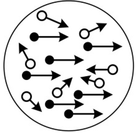
This is a famous example of a “choice reaction time” task. Not only can the response be correct or incorrect, there is also a speeded reaction time component to it. This experiment is used in all manner of psychological research, and thus it would be great if we could model the kinds of data we might expect from human (or animal) participants.

Let’s think about how we could model such a task. We’ll begin with the assumption that when the stimulus appears on the screen, participants aren’t able to answer instantly. Rather, they have to look at each dot individually, and gradually come to a conclusion about what the majority of the dots are doing. We could think of looking at each dot as gaining one new piece of evidence. If the dot is moving left, we’ll be nudged towards a conclusion that most of the dots move left, and if the dot is moving right, we’ll be nudged towards a conclusion that most of the dots are moving right.

Something like this can be modeled using a sequential sampling model. Stay with me here. We’ll assume that people sample evidence (look at dots) in discrete time steps, one at a time, and the size of that step is how much evidence is available during that step. We sum all the pieces of evidence together until some threshold is reached, and which point a decision has been reached and we can respond. This kind of model immediately gets us both responses and reaction times: what was the decision, and how long did it take before we were confident with our decision?

Let’s imagine a stimulus that is perfectly 50/50, with half the dots moving left and half the dots moving right. We’ll make the simple assumption that evidence for left nudges us in the positive direction and evidence for right nudges us in the negative direction. The evidence accumulation processes might look something like this:

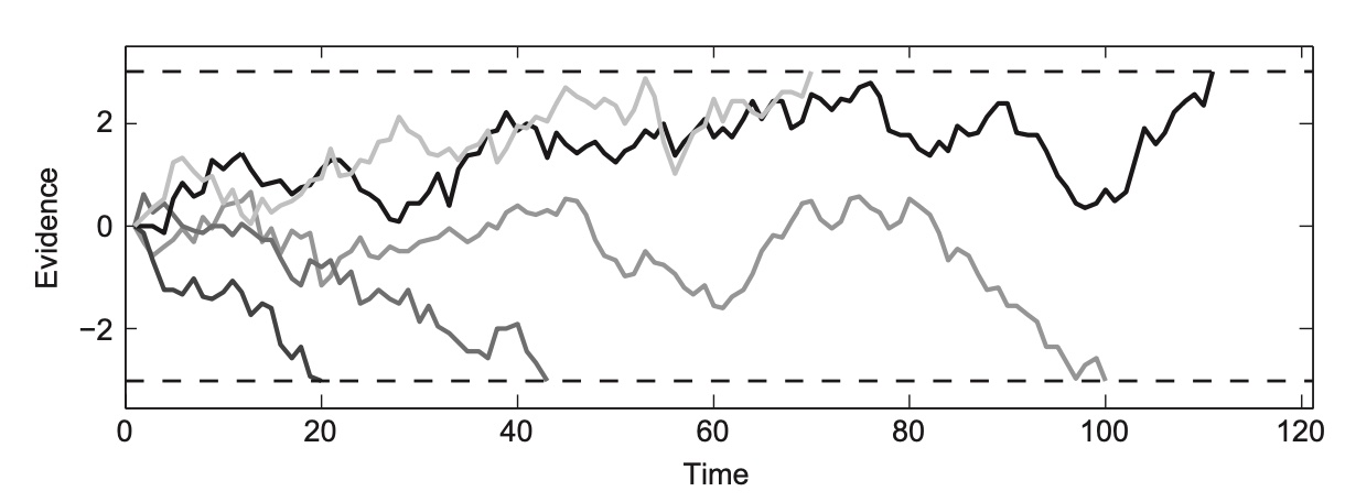
We can immediately notice a few things from these trace plots. On some trials, the nudges are almost all in the same direction, and the participant reaches a threshold where they can say “I’ve seen enough” very quickly. This might happen if 9/10 of the first dots the participant looks at are all heading towards the right. They might feel pretty comfortable pretty quickly responding with “right” without looking at the rest of the stimulus, even if they are wrong!

Some other traceplots seem to move around for a while before landing at a decision. Perhaps here the participant happened to catch enough left and right moving dots in the stimulus that they were stuck at 50/50 for a while, so they couldn’t make a decision.

This leads us to our first observation: reaction times are stochastic (random or inconsistent) even for the same stimulus!

Our second observation is that each response seems equally likely to happen, and that the reaction times for each kind of response on average should also be the same. This makes intuitive sense, since the stimulus is a 50/50 stimulus, so there should be no reason for differences in these metrics.

Next, lets imagine a stimulus whether 95% of the dots are all moving towards the left. The trajectories would look like this:

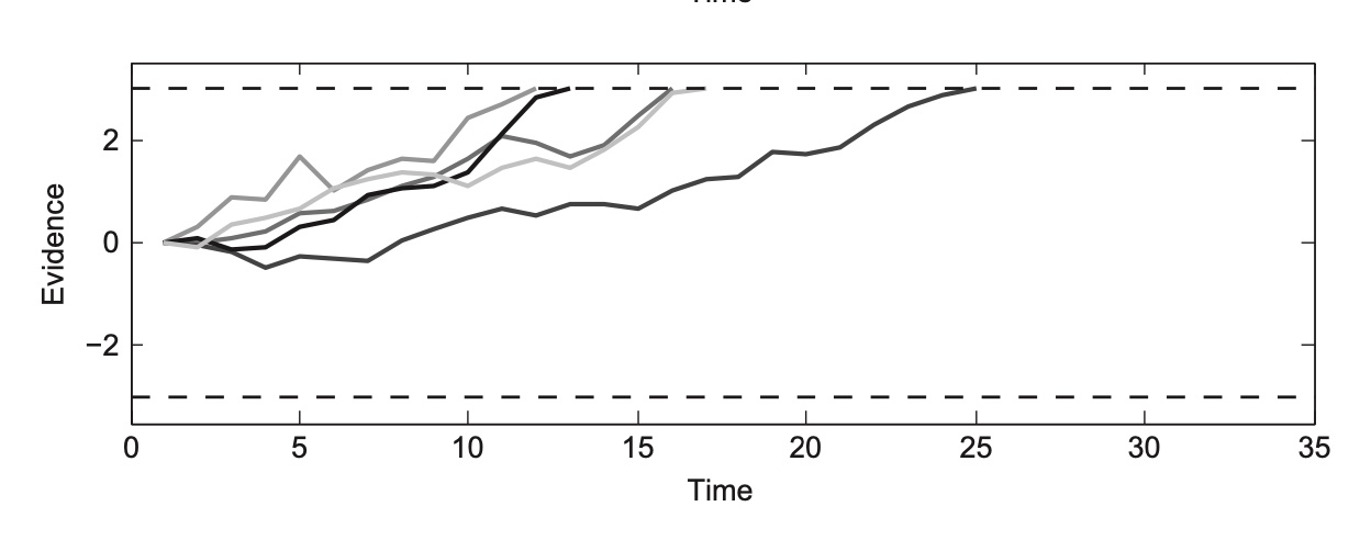
This would induce a tendency or a drift in the evidence trajectories upwards, since most of the evidence nudges us upwards. This tendency can also be called the drift rate, which in this case would be positive. We immediately see that there are no “right” responses. That is because so few dots are moving right that the probability of a person seeing 10 of those in a row is extremely unlikely. The other observation is that the reaction times are overall much faster. Since most of the dots agree, people will be able to come to a conclusion quickly.

To quote Farrell and Lewandowsky here:

“Clearly, having a highly informative stimulus permits more rapid extraction of information than staring at a non-informative stimulus that defies quick analysis.”

Building a Simulation of Our Model

Having build a rough intuition for the kinds of math we would need to model something like this, lets turn to code and actually model it. To make this even more mathematical, we’ll start with a few extra numeric assumptions. Evidence accumulation starts at 0, and at each time step, people take a “step” according to a normal distribution centered at 0. This would be the case for a neutral stimulus with 0 drift rate. They are thus equally likely to take steps in the positive or the negative direction.

Let’s write the equivalent code in R.

We’ll by defining how many trial we would like to model, and how many discrete time steps will occur on each trial.

1
2
nTrials <- 1000
nSamples <- 2000

Next, we’ll define the drift rate, which again is the tendency to randomly walk towards either of the boundaries. The larger the drift rate, the more the random walk is nudged towards a boundary. If the draft rate is 0, the walk is totally random. This corresponds to the 0 mean of the normal distribution we draw from when we take our “evidence steps”. We also specify the noise of the evidence accumulation at each step as the standard deviation of the random walk. Finally, we set the criterion, which is the threshold we need to reach before we can elicit a response, which we’ll set to an arbitrary value of 3 for now.

1
2
3
drift <- 0.0
rw_sd <- 0.3
criterion <- 3

Next, we’ll create some variables to keep track our simulation results. reaction_times and responses are both lists of length nTrials that will store the reaction time and response for each trial. We’ll initialize them with 0s for now. Finally, evidence is a nTrials x nSamples matrix that stores the evidence at each sample within a trial, also initialized as all 0s (with nSamples + 1 so that cumsum works below).

1
2
3
reaction_times <- rep(0,nTrials)
responses <- rep(0,nTrials)
evidence <- matrix(0, nTrials, nSamples + 1)

Finally, the drift process itself. For each trial, we first use the rnorm(n, mean, sd) to create a list n samples draw from a normal distribution with mean and sd. We’ll use drift and rw_sd as the mean and sd here. Using the cumsum function, we incrementally add these together, since each rnorm value reflects a “step” from the previous cumulative sum up until that point.

Once this evidence accumulation process is simulated, we simply find at which sampling point a threshold was reached (when abs(evidence) > criterion) to get our reaction time (the first time this happened, so which(abs...)[1]), and which threshold was reached tells us our response.

1
2
3
4
5
6
for (trial in c(1:nTrials)){
  evidence[trial, ] <- cumsum(c(0, rnorm(nSamples, drift, rw_sd)))
  firstPassageSample <- which(abs(evidence[trial,]) > criterion)[1]
  reaction_times[trial] <- firstPassageSample
  responses[trial] <- sign(evidence[trial, firstPassageSample])
}

And just like that, we have created a sequence of nTrials random walks! Running the code in the cell above, we can now visualize the reaction times using a histogram.

1
hist(reaction_times, breaks=50)

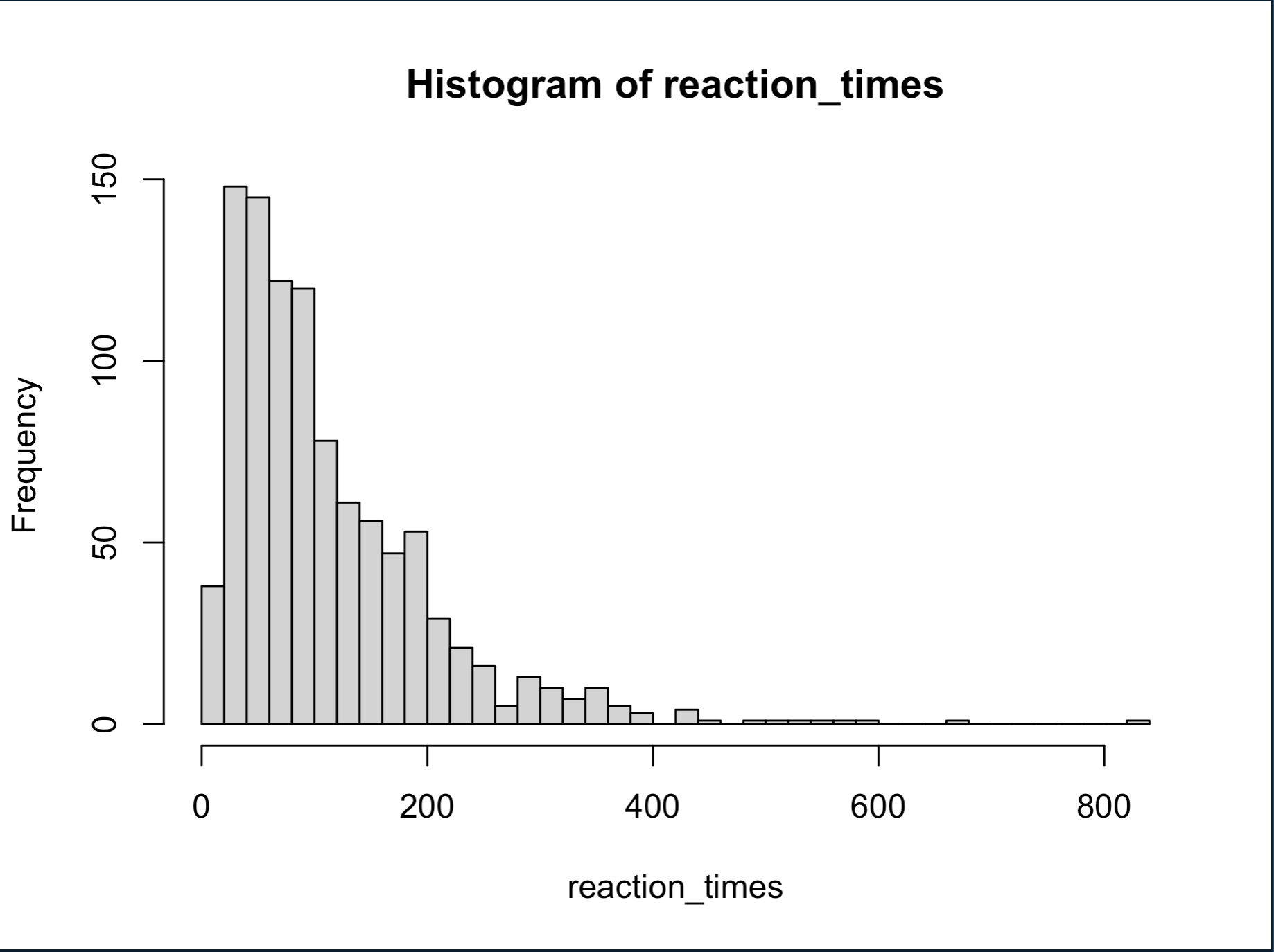
Very cool! But, of course, some of these reactions time are for different responses (left vs right). We can visualize say 5 trials worth of random walks with the following code. To briefly explain, we find the number of trials to plot (the min between nTrials and 5), then create an empty plot element with x-axis extending to fit the max of the reaction times we’re plotting (max(reaction_times[1:trialsToPlot]) and the y-axis extending to include both cutoff points ylim=c(-criterion-.5,criterion+.5). Finally we use lines to plot all trialsToPlot, cutting off at the reaction_times value (which is when the evidence exceeded the criterion). abline draws dashed horizontal lines to show our criteria.

1
2
3
4
5
6
7
8
trialsToPlot <- min(nTrials,5)
plot(1:max(reaction_times[1:trialsToPlot]),type="n",las=1,
      ylim=c(-criterion-.5,criterion+.5) ,
      ylab="Evidence",xlab="Decision time")
for (trial in c(1:trialsToPlot)) {
  lines(evidence[trial,1:(reaction_times[trial])])
}
abline(h=c(criterion,-criterion),lty="dashed")

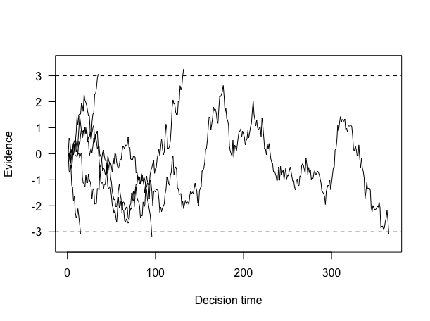
As we can now confirm, indeed some of the random walks ended up reaching the top threshold (and a “left” response was made), and some of them reached the bottom threshold (and a “right” response was made). We also have nice reaction times for how long that process took.

As we discussed earlier, with a drift rate of 0, the random walk was equally likely to reach either threshold. It makes intuitive sense that the reaction time distributions for each response to be somewhat equal. We can confirm that by plotting separate histograms for each of the two response types reaction times.

We’ll start by creating a helper function to plot histograms for us, with inputs of the data, the proportion of responses out of the whole, and the text label for the title.

1
2
3
4
5
plot_hist <- function(RT_data, RT_prop, key_word){
  hist(RT_data, col="grey", xlab="Decision Time",
       xlim = c(0, max(reaction_times)),
       main= paste(key_word, " responses (", as.numeric(RT_prop), ") m=", as.character(signif(mean(RT_data),4)),sep=""),las=1)
}

After changing a quick plotting setting, we plot both the RTs of trials for the top response (reaction_times[responses>0]) and the RTs of trials for the bottom response (reaction_times[responses<0]).

1
2
3
4
5
6
7
8
9
par(mfrow=c(2,1))

top_rt <- reaction_times[responses>0]
top_prop <- length(top_rt) / nTrials
plot_hist(top_rt, top_prop, "Top")

bot_rt <- reaction_times[responses<0]
bot_prop <- length(bot_rt) / nTrials
plot_hist(bot_rt, bot_prop, "Bottom")

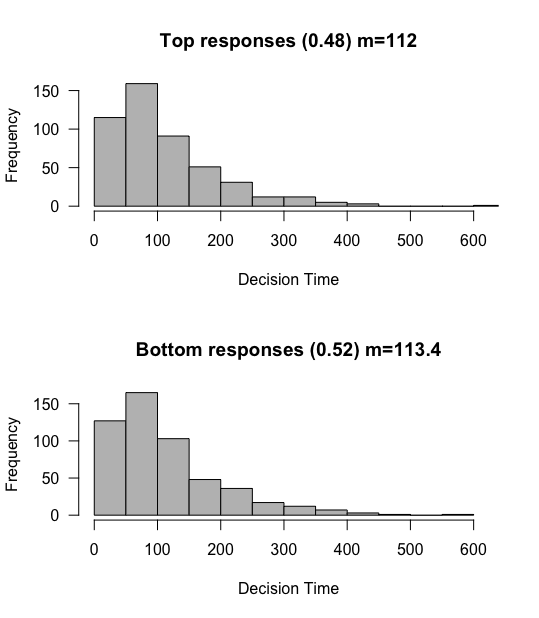
What can observe? We confirm that roughly 50% of responses tend towards to the top response, and 50% towards the bottom. The means of these distributions are also roughly the same.

Terrific! We are one step closer to a complete model of human reaction times.

Simulations

To learn more about the various parameters at stake here, lets run several simulations with different parameter values to see the effect they have on both the proportion of responses and the reaction times of each. Before we do this, we’ll define a run_simulation function that does all of the above, with inputs for the number of trials, drift rate, SD of the random walk steps, and the criterion. It returns the reaction times, the responses, and the evidence.

1
2
3
4
5
6
7
8
9
10
11
12
13
14
run_simulation <- function(nTrials, drift, rw_sd, criterion){
  reaction_times <- rep(0,nTrials)
  responses <- rep(0,nTrials)
  evidence <- matrix(0, nTrials, nSamples + 1)

  for (trial in c(1:nTrials)){
    evidence[trial, ] <- cumsum(c(0, rnorm(nSamples, drift, rw_sd)))
    firstPassageSample <- which(abs(evidence[trial,]) > criterion)[1]
    reaction_times[trial] <- firstPassageSample
    responses[trial] <- sign(evidence[trial, firstPassageSample])
  }

  return(list("RTs"=reaction_times,"Resps"=responses, "Evidence"=evidence, "nTrials"=nTrials))
}

We’ll also grab our plotting code from earlier (for the two separate histograms) and throw those into a function, with the input being the list object that the run_simulation function returns.

1
2
3
4
5
6
7
8
9
10
11
12
13
plot_simulation <- function(model_obj){
  par(mfrow=c(2,1))

  top_rt <- model_obj$RTs[model_obj$Resps>0]
  top_prop <- length(top_rt) / model_obj$nTrials
  plot_hist(top_rt, top_prop, "Top")

  bot_rt <- model_obj$RTs[model_obj$Resps<0]
  bot_prop <- length(bot_rt) / model_obj$nTrials
  plot_hist(bot_rt, bot_prop, "Bottom")

  par(mfrow=c(1,1))
}

Armed with this, we can now easily and quickly look at numerous different drift rates.

Changing the Drift Rate

Drift Rate = 0

For the first simulation, lets remind ourselves what happens when the drift rate is 0. We’ll increase the number of simulations to 10,000, so that we get more accurate estimates of the reaction time and response proportions.

1
2
sim <- run_simulation(10000, 0, 0.3, 3)
plot_simulation(sim)

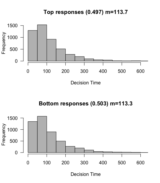
As before, we see that each threshold is reached roughly 50% of the time, with mean reaction times of about 113 “ms” (really, samples).

Drift Rate: 0 => 0.03

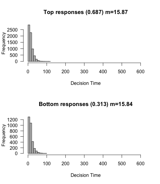
Let’s slightly increase the drift rate to 0.03

1
2
sim <- run_simulation(10000, 0.03, 0.3, 3)
plot_simulation(sim)

Two things occur, first the top response is reached more frequently, and the reaction times got faster. This makes intuitive sense for the top response, although for the bottom response less so. Shouldn’t it take longer to reach the bottom response if the tendency is upwards?

Not so! Due to the law of large numbers, longer evidence trajectories will tend to reach the upper boundary, so it is actually the very fast trajectories that make it to the bottom boundary, even though as a whole the evidence accumulation tends upwards. If there were more time, then that would just mean more opportunities for the trajectory to be nudged upwards. There are a few other details here that I will gloss over, but suffice to say we continue to expect the reaction times to be relatively equivalent.

One neat trick modelers do here is to consider the top response just “whatever is the correct response”, rather then a particular response (left or right). This lets us have a particular drift rate that gets us accuracy according to the percent of the top response. In this case we thus have an 88.7% accuracy, which is similar to what we might expect from a human participant. These two simulations therefore show us two import concepts about drift rates. Larger drift rates lead to more accurate and to faster responses.

Changing the SD of the Random Walk

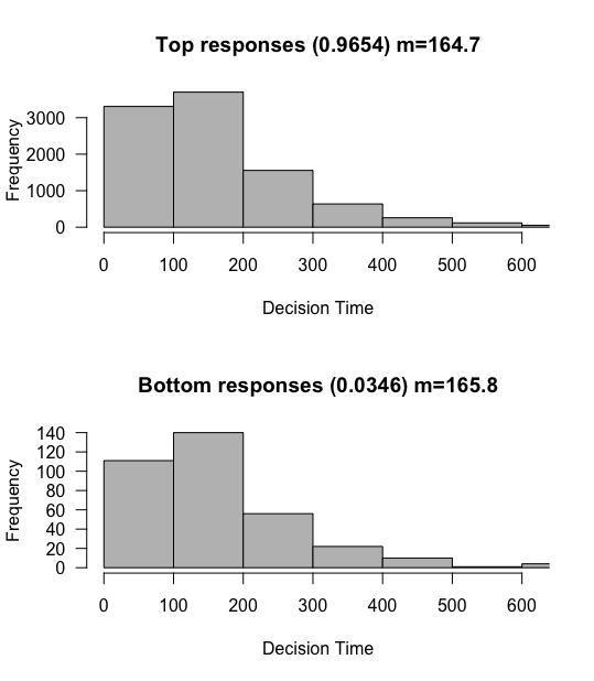
rw_sd: 0.3 => 0.5

What happens as the random walk gets noisier? Keeping the drift rate at its higher value of 0.03, lets increase the standard deviation of the random walk steps to 0.5 (from 0.3)

1
2
sim <- run_simulation(10000, 0.03, 0.5, 3)
plot_simulation(sim)

What do we observe? Reaction times as a whole get much faster, and the proportions tend back towards 50% of each. This makes intuitive sense. If you imagine a random enough process (with a wide enough SD), you would be able to reach either boundary in one step, at which point you would equally likely to reach either boundary. This would drown out the slight tendency of the mean towards one or the other boundary.

rw_sd: 0.3 => 0.1

What about when we reduce the randomness of the random walk? lets drop rw_sd to 0.1. We’ll also reduce the drift rate down to 0.01, which should make the overall proportion of each closer to 50, right?

1
2
sim <- run_simulation(10000, 0.01, 0.1, 3)
plot_simulation(sim)

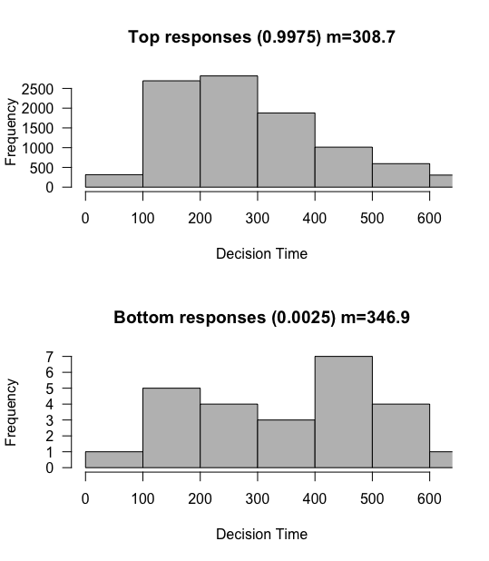
Not at all! Although yes the drift rate would make this closer to 50% if we hadn’t touched the randomness parameter, with such a stable process we actually almost universally reach the top threshold even with the reduced drift rate! That is because we are taking much smaller steps on average, and are therefore much less likely to reach the bottom threshold. By the same token, since we are taking smaller steps, the overall reaction times are much much slower, hundreds of steps slower on average in fact!

Raising the criterion

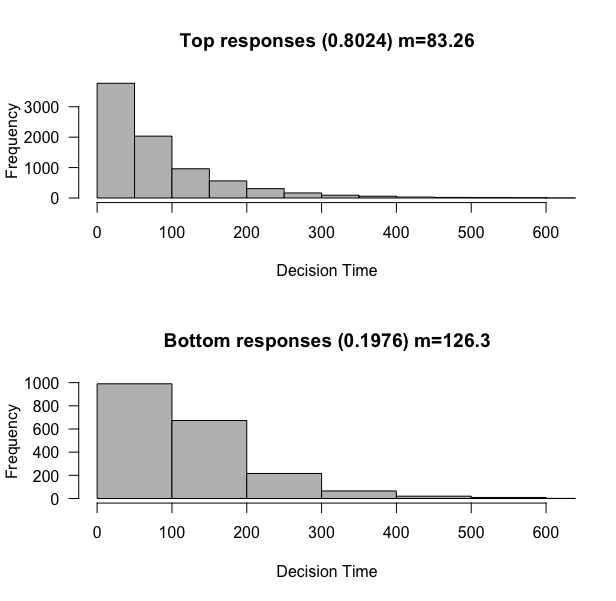
Criterion: 3 => 5

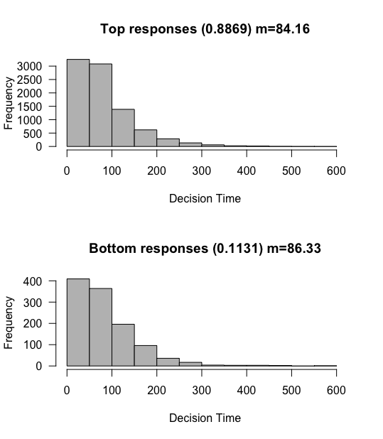
In our base simulation with a drift rate of 0.03, roughly 90% of responses were towards the top, and the reaction times were about 85 ms long. What happens if we increase the criterion? This would indicate somebody who feels they need MORE evidence before they feel comfortable responding. We’ll raise the criterion from 3 to 5.

1
2
sim <- run_simulation(10000, 0.03, 0.3, 5)
plot_simulation(sim)

Whoa! We immediately see two huge effects. First, we are even MORE likely to reach the top responses, almost 97% likely. We are also much slower. This make sense, since somebody that needs more evidence before making a decision should generally take longer on average to reach a decision. But again, we confirm that there don’t seem to be any systematic differences between reaction times between the top and bottom responses, even though one is much more likely.

Criterion: 3 => 1

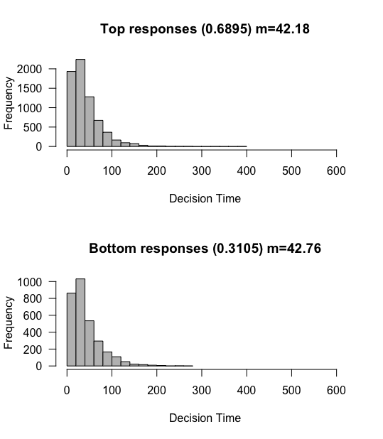
What happens if we reduce the criterion? This should correspond to someone who needs less evidence before making a response. We should expect the opposite result. People should be faster to respond, and less accurate overall.

1
2
sim <- run_simulation(10000, 0.03, 0.3, 1)
plot_simulation(sim)

Ding ding ding! Exactly. With such a short evidence criterion, people can respond really quickly, but also tend to respond more randomly since the likelihood of them reaching the incorrect threshold increases.

A new parameter, bias

Suppose 90% of the trials in our experiment were ones where the majority of dots moved towards the left. In such a situation, we might EXPECT a stimulus to be a mostly-left stimulus, even before seeing it. We would thus enter the trial with some evidence already that the stimulus will be a left-response one, even without having looked at any of the dots.

Bias: 0 => 1

To model this, we can change the cumsum function in our run_simulation function to start not at 0, but at some pre-specified value, aka the bias.

1
2
3
4
5
6
7
8
9
10
11
12
13
14
run_simulation <- function(nTrials, drift, rw_sd, criterion, bias){
  reaction_times <- rep(0,nTrials)
  responses <- rep(0,nTrials)
  evidence <- matrix(0, nTrials, nSamples + 1)

  for (trial in c(1:nTrials)){
    evidence[trial, ] <- cumsum(c(bias, rnorm(nSamples, drift, rw_sd)))
    firstPassageSample <- which(abs(evidence[trial,]) > criterion)[1]
    reaction_times[trial] <- firstPassageSample
    responses[trial] <- sign(evidence[trial, firstPassageSample])
  }

  return(list("RTs"=reaction_times,"Resps"=responses, "Evidence"=evidence, "nTrials"=nTrials))
}

Let’s run a simulation where the drift rate is 0 as in our first demo, with rw_sd 0.3 and criterion 3 as before, but with a slight bias of 1.

1
2
sim <- run_simulation(nTrials=10000, drift=0, rw_sd=0.3, criterion=3, bias=1)
plot_simulation(sim)

Even with a drift rate of 0, we tend to produce the top response. This makes sense, since we started closer to this response. We can again visualize 5 random walks to see the starting point in action here. I’ll quickly define a function to do this.

1
2
3
4
5
6
7
8
9
10
11
12
13
plot_random_walks <- function(nTrials, reaction_times, evidence, criterion, trials_to_plot){
  trialsToPlot <- min(nTrials,trials_to_plot)
  plot(1:max(reaction_times[1:trialsToPlot]),type="n",las=1,
       ylim=c(-criterion-.5,criterion+.5) ,
       ylab="Evidence",xlab="Decision time")
  for (trial in c(1:trialsToPlot)) {
    lines(evidence[trial,1:(reaction_times[trial])])
  }
  abline(h=c(criterion,-criterion),lty="dashed")
}

#call the function
plot_random_walks(sim$nTrials, sim$RTs, sim$Evidence, 3, 5)

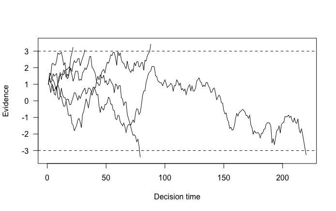
We can now clearly see how the random walks started closer to the threshold for the top response.

You might be wondering why such a manipulation results in slow errors, whereas before errors and correct responses were equally fast. Given our drift rate 0, this is simply because it takes more steps to get to the bottom threshold.

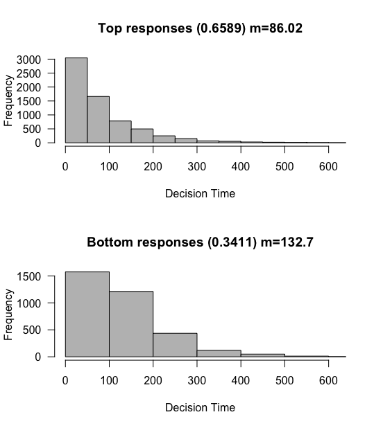
Bias: 0 => 1, but drift rate: 0 => 0.01

1
2
sim <- run_simulation(nTrials=10000, drift=0.01, rw_sd=0.3, criterion=3, bias=1)
plot_simulation(sim)

With an increased drift rate that slightly tends upward, we greatly improve our accuracy, now tending towards the top response 80% of the time. But, we maintain the fact that errors are generally slower than non-errors.

Non-Decision Time

Under our simple assumption that 1 sample roughly equals 1 ms, you may have noticed something, these reactions times are fast! A human would not be able to respond with a mean reaction time of ~85ms, although any accuracy of ~90% seems spot on. How can we change the reaction times of the data without changing the accuracy?

There is a quite simple approach to this, simply adding a flat amount of reaction time before the model is allowed to start accruing evidence towards a threshold. We call this time the non-decision time. Suppose we say that the very fastest a human could possibly respond to our dot-motion task is 300ms. Well, given that constraint, we can simply wait 300 ms before allowing the model to start drifting, which will result in the reaction times being right shifted.

Modeling this with code is quite straight forward, we simply modify the cumsum function again in our existing run_simulation function to only start sampling from the normal distribution after ndt (non-decision time) time points.

1
2
3
4
5
6
7
8
9
10
11
12
13
14
run_simulation <- function(nTrials, drift, rw_sd, criterion, bias, ndt){
  reaction_times <- rep(0,nTrials)
  responses <- rep(0,nTrials)
  evidence <- matrix(0, nTrials, nSamples + 1)

  for (trial in c(1:nTrials)){
    evidence[trial, ] <- cumsum(c(bias, rep(0, ndt), rnorm(nSamples - ndt, drift, rw_sd)))
    firstPassageSample <- which(abs(evidence[trial,]) > criterion)[1]
    reaction_times[trial] <- firstPassageSample
    responses[trial] <- sign(evidence[trial, firstPassageSample])
  }

  return(list("RTs"=reaction_times,"Resps"=responses, "Evidence"=evidence, "nTrials"=nTrials))
}

Let’s run this simulation with a non decision time of 300 ms, for a very accurate participant with drift 0.03 that is unbiased.

1
2
sim <- run_simulation(nTrials=10000, drift=0.03, rw_sd=0.3, criterion=3, bias=0, ndt=300)
plot_simulation(sim)

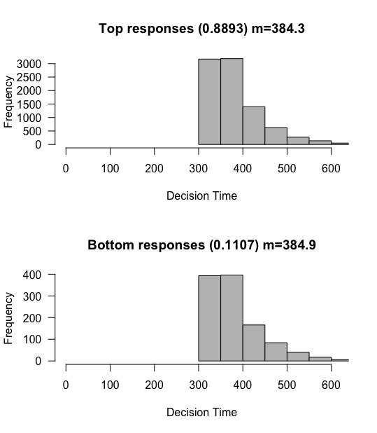
What do we notice? Although the overall proportions dont change, the mean reaction times are shifted by exactly 300 ms!

Summarizing our parameters

We have seen several “parameters” or changeable levers in our math model, reviewed below.

• Drift: the tendency towards the upper or lower boundaries, with larger values leading to faster and more accurate responses.
• Randomness of Walk: how noisy our steps are.
• Criterion: how much evidence is needed before we are confident responding? Also known as the response threshold.
• Bias: Whether we start with a predisposition towards one of the responses.
• Non Decision Time: Time before the drifting begins. In psychology, this might reflect basic visual processing (in the retina for example) that needs to occur BEFORE we can start looking at dots and collecting evidence.

We have just built what psychologists refer to as a drift diffusion model! There are many other versions of this. The “full” DDM (also known as the Ratcliffe DDM) has even more parameters, with noise for each of the parameters above. Thus, the drift can vary from trial to trial, the bias can vary from trial to trial, the non decision time can vary from trial to trial, etc. Each of these parameters has an additional parameter that specified the variance of these parameters.

On the other side, one of the most widely used DDMs is the Wiener diffusion model, which assumes fixed “randomness” and therefore just has 4 parameters: dirft rate, bias, non-decision time, and the response threshold (criterion).

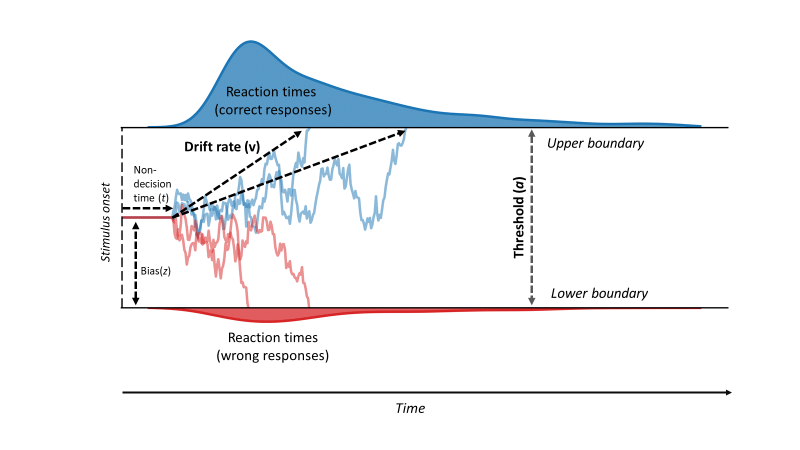
Below is Figure 2 of a DDM from Vinding et al., 2018 that I randomly found on the internet.

As we can see, we are now familiar with all of these parameters! They are often made a little harder to understand by giving them those little letter representations, but the logic is all the same.

Parameter Estimation of DDMs

TBD!