Signal detection in math and psychology

When we are thinking about signal detection, we typically are concerened with separating between some signal and noise. In an experiment, on each trial, we have a signal that may or may not be present. At each point, noise is added to create the stimulus. Then this goes through a detector – sometimes a machine learning algorithm, sometimes a human being – to decide if the signal is present or not.

In recognition tasks, we often expose people to novel and seen before stimuli. The novel stimuli are the noise and those they have seen before are the signal. They themselves are the detector, and are the ones to decide if signal is present or not. We want to be able to say something about their sensitivity to stimuli and their bias in these tasks, and for that we turn to signal detection theory! In psychology, this type of terminology originated in perception tasks, where many of these terms make a lot of sense too - in recognition/memory tasks, the signal and noise are more internal, whereas in perception tasks the signal and noise are mainly external.

We’re generally interested in a couple things: first, a participant’s sensitivity to the signal (indicated by how often they correctly say that a signal is present). This is also a measure of how ‘strong’ their signal distribution is, or how distinct it is from their noise distribution. In other words, how easy is it for participants to tell that they’ve seen a stimulus before?

We’re also interested in a participant’s bias, or propensity to say yes. This is also known as the criterion (which will be marked as c). We can estimate both of these properties by asking participants simple yes/no questions (“have you seen this stimulus before?”), and then using R to analyze the data!

CREDIT CREDIT CREDIT

the examples and code from this tutorial come from this tutorial, which Kevin sent me, and the thoughts and words come from my brain and class notes. THE CODE IS NOT MINE! i am dusting off R for the first time in a literal year

Terms and notation

When thinking about Detecting Signals, there are four possible outcomes of our Signal Detection: 1. There could be a signal, and we could detect it (a hit) 2. There could be a signal, and we could not detect it (a miss) 3. There could be no signal, and we could say there is no signal (a correct rejection,or CR) 4. There could be no signal, and we could think there’s a signal (a false positive, or FP)

There are therefore a few values we’re interested in: The probability our participants were correct:

The probability that our participants were wrong:

The hit rate:

The FP rate:

The hit rate and false positive rate are particularly important, because they tell us about where our signal distribution is and where our detection criterion is. The way people typically think about this is in terms of two overlapping Gaussian distributions, like here:

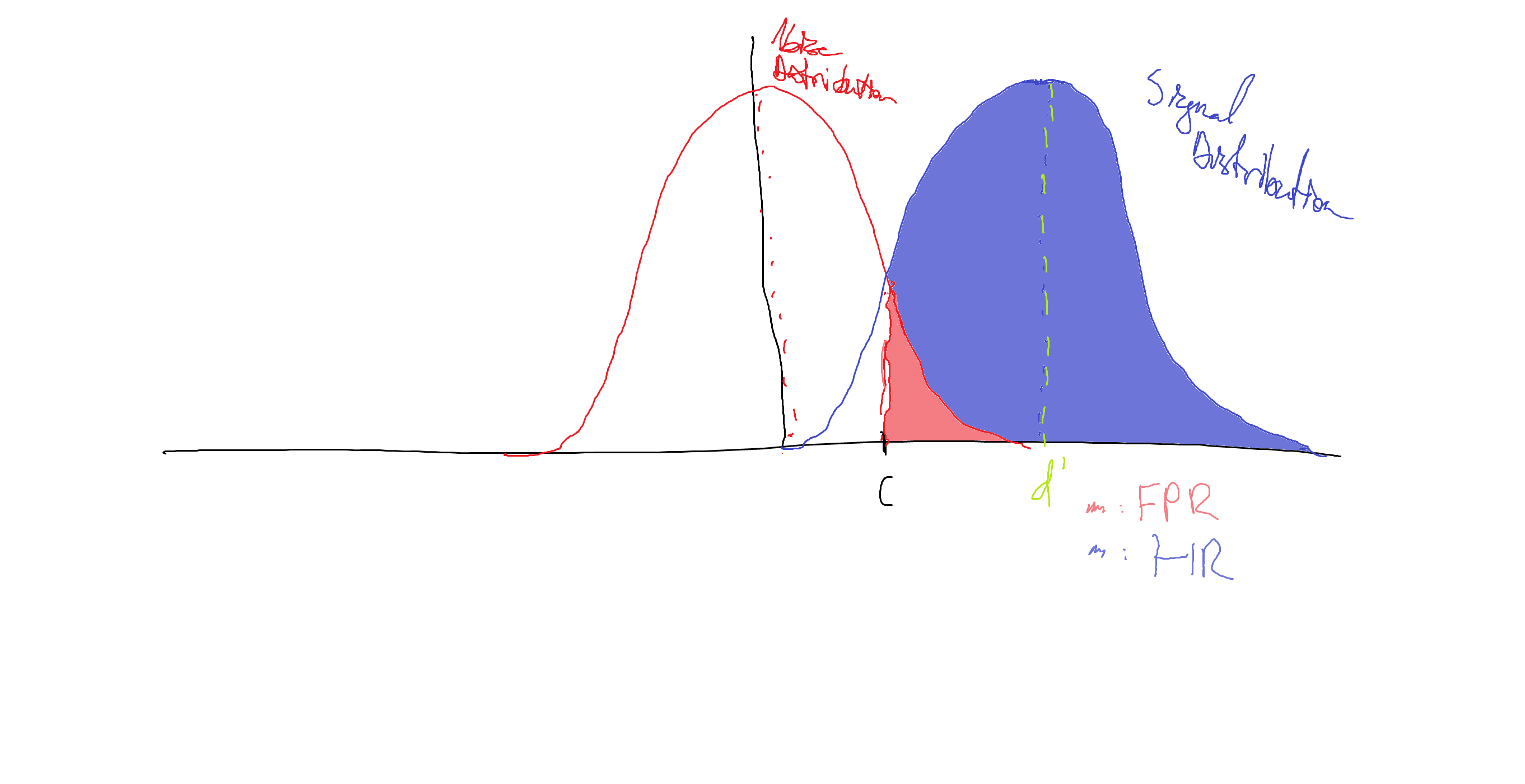
The red Gaussian is our noise distribution - thought to be centered at zero intensity (has a mean of zero).

The blue Gaussian is our signal distribution. It has some positive mean, indicated by d’. The shaded region of the blue Gaussian indicates the area of the signal distribution above our decision criterion, c. This area is equivalent to the probability that we say that there is a signal given that we see a signal, a.k.a. our HR. The shaded region of the red Gaussian is the area of the noise distribution above our criterion, equivalent to our FPR.

Equal Variance Gaussian Model

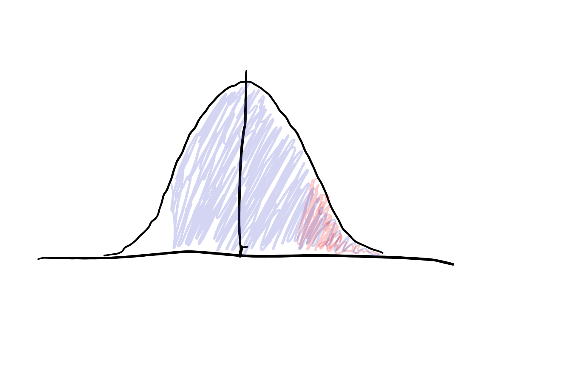
Given this framework, we actually already have everything we need to start to estimate each participant’s sensitivity and bias. In the Equal Variance Gaussian model, our noise and signal distributions are assumed to be Gaussians with unit variance and different means. This is the model we’ll cover today! If you’re interested in more complex things we can do that in the future. Under this framework, the noise distribution is a standard normal, and the d’ we estimate is the distance, measured in standard deviations, of the mean of our signal distribution from the mean of the noise distribution.

If we shift the signal distribution over by d’, we can overlay the signal and noise distributions, since their variances are assumed equal.

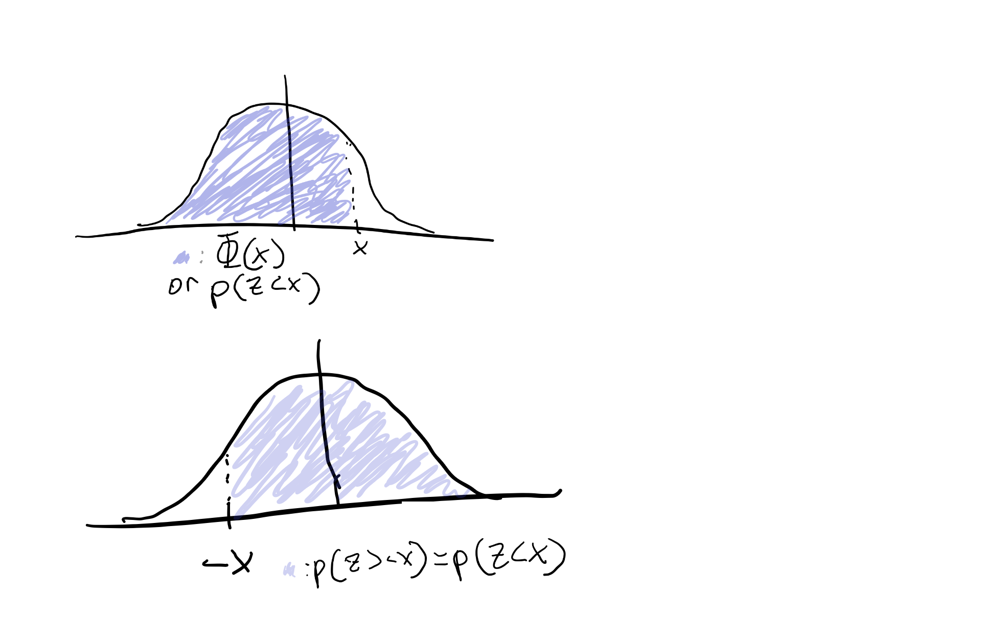
We can then use some helpful properties of the Gaussian distribution to help us figure out what d’ and c are. We have our HR and FPR indicated above, and since these come from standard normal distributions, we can use the cumulative density function (CDF) indicated by \( \Phi\), to describe our HR and FPR. The CDF of a distribution, \(\Phi(x)\), is the area under our distribution less than or equal to x, or the probability that we see a value drawn from our distribution less than or equal to x. Since Gaussians are symmetric around their mean, we ALSO know that \(P(x < z) = P(x > -z)\) (see figure below)

We can use this sneaky trick to say the following:

Our HR is the probability our signal distribution lays to the right of our criterion. Since we shifted our signal distribution to the right by subtracting d’, this is the same as the probability a standard normal is greater than c - d’. Reversing this, this is finally equivalent to the probability a standard normal is LESS than d’ - c.

Since we did not shift our noise distribution at all, and again that distribution is symmetric. The inverse of this function, \(\Phi^{-1}(x)\), exists also and I’m not gonna draw it out or say anything more than that it exists so please just believe me. Given this, we know that

So we have our criterion from our FPR! If we subtract the right half from the left half, our c’s cancel and we get back d’, giving

Thanks for sitting through me through this math! Now we can do this in R. The link linked in the first section has this code so if you want another explanation go there!Libraries used:

1
2
3
4
5
6
7
library(knitr)
library(scales)
library(bayesplot)
library(ggridges)
library(sdtalt)
library(brms)
library(tidyverse)

Data used, from the sdtalt package and Wright 2011 ¹:

We first need to find what kind of trial each trial was (Hit, FP, CR, or miss). We can do this doing the following:

1
2
3
4
5
6
7
sdt <- confcontr %>%
    mutate(
        type="hit",
        type = ifelse(isold == 1 & sayold == 0, "miss",type),
        type = ifelse(isold == 0 & sayold==0, "cr",type),
        type=ifelse(isold == 0 & sayold == 1, "fp", type)
    )

These lines of code create a new “type” variable that codes for what trial type our participants ended up giving us. We can then format this for each participant to give us one row per participant, so we can find hit rates, FPRs, etc.

1
2
3
4
sdt <- sdt %>%
    group_by(subno,type) %>%
    summarise(count=n()) %>%
    spread(type,count) #formats to one row per participant

R has a nice function to let us calculate $\Phi^{-1}(x)$, qnorm(). Using this to calculate d’, c:

1
2
3
4
5
6
7
8
9
sdt <- sdt %>%
    mutate(
        zhr = qnorm(hit/(hit + miss)),
        zfp = qnorm(fp/(fp + cr)),
        dprime = zhr - zfp,
        crit = -zfp
    )

kable(sdt[1:5, ], caption = "Point estimates of d', c")

Point estimates of d’, c

Yay! This is great this gives estimates for our quantities of interest, d’ and c. But there are other ways we can look at this!

Estimating Equal Variance Gaussian model with GLM

You’ve seen our point estimates (above), which give us the most likely parameter estimates for our model - there, we are using a frequentist perspective to estimate our parameters. We can approach this from a more Bayesian perspective, however.

We can model probabilities using logistic regression models, in these models, we model our outcomes as binary (1 if participants say they’d seen a stimulus before, 0 otherwise). These assume that each trial is independently drawn from a Bernoulli distribution, with the probability of a trial being a 1 set to \(p\). We can model \(p\) as \(\Phi(\eta)\) - again, the probability that a standard normal distribution is less than \(\eta\). We then get to choose how we model \(\eta\), based on our data. Our life is made simpler if we choose a linear relationship between our data and \(\eta\): \(\eta = \beta_0 + \beta_1 * \text{stimulus seen}\). This parameterization gives us a good interpretation for these parameters. Let’s say the simulus is new, which means that stimulus_seen = 0. Our interpretation for \(p\) here is our FPR: the probability of saying we’ve seen a stimulus, when we in fact have not. Then \(\eta\) = \(\beta_0\), and \(FPR = \Phi(\beta_0)\). This looks familiar to what we had above, which what \(FPR = \Phi(-c)\). When stimulus_seen = 1, our \(p\) is the probability of getting a hit, or our HR. From above, we have \(HR = \Phi(d’ - c)\). This trial type gives \(\eta = -c + \beta_1\), so \(d’ = \beta_1\)! How nice. We can fit this on an individual subjects level doing the following:

1
2
3
4
5
6
7
evsdt_1 <- brm(
  sayold ~ isold,
  family = bernoulli(link="probit"),
  data = filter(confcontr,subno == 53),
  cores = 4,
  file="sdtmodel1-1"
)

This framework uses the BAYESIAN REGRESSION MODELING package brms! This is wonderful since brms extends to complicated frameworks in the future. It saves the model in evsdt_1, and we can get a summary of what’s going on here with this:

1
summary(evsdt_1)

1
2
3
4
5
6
7
8
9
10
11
12
13
14
15
##  Family: bernoulli 
##   Links: mu = probit 
## Formula: sayold ~ isold 
##    Data: filter(confcontr, subno == 53) (Number of observations: 100) 
##   Draws: 4 chains, each with iter = 2000; warmup = 1000; thin = 1;
##          total post-warmup draws = 4000
## 
## Population-Level Effects: 
##           Estimate Est.Error l-95% CI u-95% CI Rhat Bulk_ESS Tail_ESS
## Intercept    -0.32      0.17    -0.66     0.02 1.00     3250     2605
## isold         0.39      0.25    -0.10     0.90 1.00     3532     2566
## 
## Draws were sampled using sampling(NUTS). For each parameter, Bulk_ESS
## and Tail_ESS are effective sample size measures, and Rhat is the potential
## scale reduction factor on split chains (at convergence, Rhat = 1).

we can then visualize this using the following:

1
2
3
4
5
6
7
8
9
posterior <- as.array(evsdt_1)


scatter_dprime_c <- mcmc_scatter(
  posterior,
  pars=c("b_Intercept","b_isold"),
  size=1
)
scatter_dprime_c

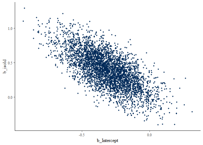
There are PROBABLY better ways to look at these, but this is what I have chosen! Here, b_isold is \(\beta_1\), or d’, while b_Intercept is -c.

Nonlinear Equal Variance Gaussian Model

We can additionally make this model nonlinear to directly estimate c and d’. Specifically, instead of estimating \(\eta\), we can write:

This looks the same as before, but is directly estimating these two parameters. This makes things a bit more complicated, so we can use a nonlinear model! Specifying this model can be done with similar syntax to before:

1
2
3
4
5
nonlinear_model <- bf(
    sayold ~ Phi(dprime * isold - c),
    dprime ~ 1, c ~ 1,
    nl=TRUE
)

This code is first, detailing the relationship between the probability our participants said a stimulus was old (sayold ~ Phi(dprime * isold - c)).

The second line tells the model to estimate both dprime and c (dprime ~ 1, c ~ 1). The third line says that the model is nonlinear. This is a more difficult problem to solve (in general), so the package used by this one guy requires us to set priors on dprime and c, using the following lines of code:

1
2
3
4
Priors <- c(
  prior(normal(.5, 3), nlpar = "dprime"),
  prior(normal(0, 1.5), nlpar = "c")
)

Finally, we can estimate our model! We can do this for each participant. It’s again using brm, as follows:

1
2
3
4
5
6
7
8
9
evsdt_2 <- brm(
  nonlinear_model,
  family = bernoulli(link = "identity"),
  data = filter(confcontr, subno == 53),
  prior = Priors,
  control = list(adapt_delta = .99),
  cores = 4,
  file = "sdtmodel1-2"
)

Here, the link function is the identity because our model is already nonlinear- we don’t need to introduce a link function.

Then we can compare the first model and the second model!

1
2
3
4
5
6
7
8
9
10
11
12
13
14
15
16
17
18
19
20
21
22
23
24
25
26
27
28
29
30
31
32
33
34
35
36
37
evsdt_1:

##  Family: bernoulli 
##   Links: mu = probit 
## Formula: sayold ~ isold 
##    Data: filter(confcontr, subno == 53) (Number of observations: 100) 
##   Draws: 4 chains, each with iter = 2000; warmup = 1000; thin = 1;
##          total post-warmup draws = 4000
## 
## Population-Level Effects: 
##           Estimate Est.Error l-95% CI u-95% CI Rhat Bulk_ESS Tail_ESS
## Intercept    -0.32      0.17    -0.66     0.02 1.00     3250     2605
## isold         0.39      0.25    -0.10     0.90 1.00     3532     2566
## 
## Draws were sampled using sampling(NUTS). For each parameter, Bulk_ESS
## and Tail_ESS are effective sample size measures, and Rhat is the potential
## scale reduction factor on split chains (at convergence, Rhat = 1).

evsdt_2:

##  Family: bernoulli 
##   Links: mu = identity 
## Formula: sayold ~ Phi(dprime * isold - c) 
##          dprime ~ 1
##          c ~ 1
##    Data: filter(confcontr, subno == 53) (Number of observations: 100) 
##   Draws: 4 chains, each with iter = 2000; warmup = 1000; thin = 1;
##          total post-warmup draws = 4000
## 
## Population-Level Effects: 
##                  Estimate Est.Error l-95% CI u-95% CI Rhat Bulk_ESS Tail_ESS
## dprime_Intercept     0.40      0.25    -0.10     0.88 1.00     1231     1418
## c_Intercept          0.31      0.18    -0.04     0.66 1.00     1099     1306
## 
## Draws were sampled using sampling(NUTS). For each parameter, Bulk_ESS
## and Tail_ESS are effective sample size measures, and Rhat is the potential
## scale reduction factor on split chains (at convergence, Rhat = 1).

These give roughly the same results, but it can be useful in other situations to use a more complex model to fit data - and this is a way to do that.

Multiple participants estimation

To model multiple participants, you can either summarize the point estimates OR estimate a hierarchical model.

Summarizing point estimates

Since we calculated d’ and c for all of our participants, we can summarize those to give us a mean and standard deviation for each parameter:

1
2
3
4
sdt_sum <- select(sdt,subno,dprime,crit) %>%
  gather(parameter,value,-subno) %>%
  group_by(parameter) %>%
  summarise(n = n(),mu=mean(value),sd=sd(value),se=sd/sqrt(n))

This gives us average values, standard deviations, and standard errors for our parameter estimates across our population. Then we can run t-tests and the sort on this stuff!

Hierarchical modeling

We could ALSO use a hierarchical model, in which we modify the logistic regression from above: we fit a logistic model for each participant, with the participant-specific parameters drawn from a multivariate normal distribution:

This gives us a model where we have an estimate for each participant, but also an estimate of each parameter “for the average participant”. It also tells us about the variance of each parameter and the covariance between parameters, which in turn give us standard deviations and correlations. Standard deviations for each parameter tell us about typical variance in the population, and correlations tell us about the typical relationship between d’ and c. In order to fully specify this model, we need to estimate 5 parameters on the population level: \(\mu_1\), \(\mu_2\), \(\mathbb{V}[\beta_0]\), \(\mathbb{V}[\beta_1]\), and covar\((\beta_0,\beta_1)\).

We can again use brms to build these models. The formula looks a bit different, but the overall model is the same:

1
2
3
4
5
6
evsdt_glmm <- brm(sayold ~ 1 + isold + (1 + isold | subno),
  family = bernoulli(link = "probit"),
  data = confcontr,
  cores = 4,
  file = "sdtmodel2-1"
)

The part of the formula outside of the parentheses specifies that we want to estimate the mean intercept and mean slope for all participants, and the part within the parentheses says that we want to estimative the variance and covariance of those parameters across participants.

Again, the intercept is our -c, and the slope is d’. We can then compare these estimates to our manual estimates across our population!

1
2
3
4
5
6
7
8
9
10
11
12
13
14
15
16
17
18
19
20
21
22
23
24
25
26
##  Family: bernoulli 
##   Links: mu = probit 
## Formula: sayold ~ 1 + isold + (1 + isold | subno) 
##    Data: confcontr (Number of observations: 3100) 
##   Draws: 4 chains, each with iter = 2000; warmup = 1000; thin = 1;
##          total post-warmup draws = 4000
## 
## Group-Level Effects: 
## ~subno (Number of levels: 31) 
##                      Estimate Est.Error l-95% CI u-95% CI Rhat Bulk_ESS
## sd(Intercept)            0.26      0.05     0.16     0.38 1.00     1612
## sd(isold)                0.38      0.08     0.24     0.56 1.00     1062
## cor(Intercept,isold)    -0.57      0.18    -0.84    -0.13 1.00     1135
##                      Tail_ESS
## sd(Intercept)            2358
## sd(isold)                2098
## cor(Intercept,isold)     1619
## 
## Population-Level Effects: 
##           Estimate Est.Error l-95% CI u-95% CI Rhat Bulk_ESS Tail_ESS
## Intercept    -0.66      0.06    -0.77    -0.54 1.00     1968     1894
## isold         1.06      0.09     0.89     1.23 1.00     1677     2196
## 
## Draws were sampled using sampling(NUTS). For each parameter, Bulk_ESS
## and Tail_ESS are effective sample size measures, and Rhat is the potential
## scale reduction factor on split chains (at convergence, Rhat = 1).

By looking at this, we can see that on average our estimates are the same between these two methods, but the manual calculation method estimates a higher standard deviation for these parameters among our participants! That’s pretty neat.

Anyway, overall these are a few different methods of estimating sensitivity and bias in recognition tasks, whether they be memory-based or psychophysics based! If you have any more questions! please ask me.

frame this ENTIRELY differently, draw some graphs yourself. you are selling this to a cogneuro crowd, so you don’t actually NEED very much SDT. you just need to justify what d’, c are, then tell use why different versions of this matter.

There are PROBABLY better ways to look at these, but this is what I have chosen! Here, b_isold is \(\beta_1\), or d’, while b_Intercept is -c.

Nonlinear Equal Variance Gaussian Model

We can additionally make this model nonlinear to directly estimate c and d’. Specifically, instead of estimating \(\eta\), we can write:

This looks the same as before, but is directly estimating these two parameters. This makes things a bit more complicated, so we can use a nonlinear model! Specifying this model can be done with similar syntax to before:

1
2
3
4
5
nonlinear_model <- bf(
    sayold ~ Phi(dprime * isold - c),
    dprime ~ 1, c ~ 1,
    nl=TRUE
)

This code is first, detailing the relationship between the probability our participants said a stimulus was old (sayold ~ Phi(dprime * isold - c)).

The second line tells the model to estimate both dprime and c (dprime ~ 1, c ~ 1). The third line says that the model is nonlinear. This is a more difficult problem to solve (in general), so the package used by this one guy requires us to set priors on dprime and c, using the following lines of code:

1
2
3
4
Priors <- c(
  prior(normal(.5, 3), nlpar = "dprime"),
  prior(normal(0, 1.5), nlpar = "c")
)

Finally, we can estimate our model! We can do this for each participant. It’s again using brm, as follows:

1
2
3
4
5
6
7
8
9
evsdt_2 <- brm(
  nonlinear_model,
  family = bernoulli(link = "identity"),
  data = filter(confcontr, subno == 53),
  prior = Priors,
  control = list(adapt_delta = .99),
  cores = 4,
  file = "sdtmodel1-2"
)

Here, the link function is the identity because our model is already nonlinear- we don’t need to introduce a link function.

Then we can compare the first model and the second model!

1
2
3
4
5
6
7
8
9
10
11
12
13
14
15
16
17
18
19
20
21
22
23
24
25
26
27
28
29
30
31
32
33
34
35
36
37
evsdt_1:

##  Family: bernoulli 
##   Links: mu = probit 
## Formula: sayold ~ isold 
##    Data: filter(confcontr, subno == 53) (Number of observations: 100) 
##   Draws: 4 chains, each with iter = 2000; warmup = 1000; thin = 1;
##          total post-warmup draws = 4000
## 
## Population-Level Effects: 
##           Estimate Est.Error l-95% CI u-95% CI Rhat Bulk_ESS Tail_ESS
## Intercept    -0.32      0.17    -0.66     0.02 1.00     3250     2605
## isold         0.39      0.25    -0.10     0.90 1.00     3532     2566
## 
## Draws were sampled using sampling(NUTS). For each parameter, Bulk_ESS
## and Tail_ESS are effective sample size measures, and Rhat is the potential
## scale reduction factor on split chains (at convergence, Rhat = 1).

evsdt_2:

##  Family: bernoulli 
##   Links: mu = identity 
## Formula: sayold ~ Phi(dprime * isold - c) 
##          dprime ~ 1
##          c ~ 1
##    Data: filter(confcontr, subno == 53) (Number of observations: 100) 
##   Draws: 4 chains, each with iter = 2000; warmup = 1000; thin = 1;
##          total post-warmup draws = 4000
## 
## Population-Level Effects: 
##                  Estimate Est.Error l-95% CI u-95% CI Rhat Bulk_ESS Tail_ESS
## dprime_Intercept     0.40      0.25    -0.10     0.88 1.00     1231     1418
## c_Intercept          0.31      0.18    -0.04     0.66 1.00     1099     1306
## 
## Draws were sampled using sampling(NUTS). For each parameter, Bulk_ESS
## and Tail_ESS are effective sample size measures, and Rhat is the potential
## scale reduction factor on split chains (at convergence, Rhat = 1).

These give roughly the same results, but it can be useful in other situations to use a more complex model to fit data - and this is a way to do that.

Multiple participants estimation

To model multiple participants, you can either summarize the point estimates OR estimate a hierarchical model.

Summarizing point estimates

Since we calculated d’ and c for all of our participants, we can summarize those to give us a mean and standard deviation for each parameter:

1
2
3
4
sdt_sum <- select(sdt,subno,dprime,crit) %>%
  gather(parameter,value,-subno) %>%
  group_by(parameter) %>%
  summarise(n = n(),mu=mean(value),sd=sd(value),se=sd/sqrt(n))

This gives us average values, standard deviations, and standard errors for our parameter estimates across our population. Then we can run t-tests and the sort on this stuff!

Hierarchical modeling

We could ALSO use a hierarchical model, in which we modify the logistic regression from above: we fit a logistic model for each participant, with the participant-specific parameters drawn from a multivariate normal distribution:

This gives us a model where we have an estimate for each participant, but also an estimate of each parameter “for the average participant”. It also tells us about the variance of each parameter and the covariance between parameters, which in turn give us standard deviations and correlations. Standard deviations for each parameter tell us about typical variance in the population, and correlations tell us about the typical relationship between d’ and c. In order to fully specify this model, we need to estimate 5 parameters on the population level: \(\mu_1\), \(\mu_2\), \(\mathbb{V}[\beta_0]\), \(\mathbb{V}[\beta_1]\), and covar\((\beta_0,\beta_1)\).

We can again use brms to build these models. The formula looks a bit different, but the overall model is the same:

1
2
3
4
5
6
evsdt_glmm <- brm(sayold ~ 1 + isold + (1 + isold | subno),
  family = bernoulli(link = "probit"),
  data = confcontr,
  cores = 4,
  file = "sdtmodel2-1"
)

The part of the formula outside of the parentheses specifies that we want to estimate the mean intercept and mean slope for all participants, and the part within the parentheses says that we want to estimative the variance and covariance of those parameters across participants.

Again, the intercept is our -c, and the slope is d’. We can then compare these estimates to our manual estimates across our population!

1
2
3
4
5
6
7
8
9
10
11
12
13
14
15
16
17
18
19
20
21
22
23
24
25
26
##  Family: bernoulli 
##   Links: mu = probit 
## Formula: sayold ~ 1 + isold + (1 + isold | subno) 
##    Data: confcontr (Number of observations: 3100) 
##   Draws: 4 chains, each with iter = 2000; warmup = 1000; thin = 1;
##          total post-warmup draws = 4000
## 
## Group-Level Effects: 
## ~subno (Number of levels: 31) 
##                      Estimate Est.Error l-95% CI u-95% CI Rhat Bulk_ESS
## sd(Intercept)            0.26      0.05     0.16     0.38 1.00     1612
## sd(isold)                0.38      0.08     0.24     0.56 1.00     1062
## cor(Intercept,isold)    -0.57      0.18    -0.84    -0.13 1.00     1135
##                      Tail_ESS
## sd(Intercept)            2358
## sd(isold)                2098
## cor(Intercept,isold)     1619
## 
## Population-Level Effects: 
##           Estimate Est.Error l-95% CI u-95% CI Rhat Bulk_ESS Tail_ESS
## Intercept    -0.66      0.06    -0.77    -0.54 1.00     1968     1894
## isold         1.06      0.09     0.89     1.23 1.00     1677     2196
## 
## Draws were sampled using sampling(NUTS). For each parameter, Bulk_ESS
## and Tail_ESS are effective sample size measures, and Rhat is the potential
## scale reduction factor on split chains (at convergence, Rhat = 1).

By looking at this, we can see that on average our estimates are the same between these two methods, but the manual calculation method estimates a higher standard deviation for these parameters among our participants! That’s pretty neat.

Anyway, overall these are a few different methods of estimating sensitivity and bias in recognition tasks, whether they be memory-based or psychophysics based! If you have any more questions! please ask me.

frame this ENTIRELY differently, draw some graphs yourself. you are selling this to a cogneuro crowd, so you don’t actually NEED very much SDT. you just need to justify what d’, c are, then tell use why different versions of this matter.