
Linear Regression (The basics)

You’ve probably come across linear regression from time to time in your research, or in reading papers – but how does it work? What is linear regression? What are the assumptions behind it? How do I do it? We’re going to hit on the basics of all those questions in this tutorial right here.
Table of Contents
- Introduction: What is linear regression?
- Linear regression how-tos:
- How to set up your data
- How to code your model
- sklearn
- statsmodels
- Interpreting Linear Regression
What is linear regression?
A way of modeling relationships between variables
Oftentimes in our research, we’re interested in understanding the relationship between independent variables and dependent variables. Linear regression lets us describe that relationship! It’s just one of many ways of modeling relationships, but in many ways is one of the simplest, easiest to implement, most commonly found, and is usually: good enough for all your modeling needs.
Linear regression form
For the form of linear regression, we’re going to reach back into our memories and bring back slope-intercept form from our geometry classes back in the day. For a refresher, slope-intercept is:
y = mx + b
Where m is the slope, and b is the intercept. In our linear regression, x is our independent variable, or our predictor, and y is our dependent variable, or outcome. We’re modeling the relationship between the two as linear: assuming that you can draw a straight line to relate predictors to outcomes. In research & modeling, the slope and intercept are typically known as β weights, and the above formula is written as:
y = β1x + β0
Because of this, we’ll be using β to mark and describe our linear regression weights
When should we use linear regression?
Linear regression is a great tool for a lot of things - if we’re just starting a new set of data analysis, basic linear regression can be a way to explore relationships in our data. If we’re deeper in our analyses, we can use linear regression to test if linear relationships exist in our data. We can use this for both continuous and categorical predictors. However, if we have categorical output variables, there are usually better options (that I won’t cover here, but you can look up logistic regression and multinomial regression if you want more information)
How does linear regression work?
I said before that linear regression models the relationship between predictors and outcomes - but how does it do that? How does it find our slope-intercept form? It does so by finding the slope and intercept that minimize error between predictions and true outcomes. We have our estimate:
ŷ = β1x + β0
and the best values of β1, β0 are those that minimize (ŷ−y)2. If we have multiple data points (as we usually do in most datasets), linear regression minimizes that error on average across the whole dataset.
but what happens if there isn’t a linear relationship in our data? what does linear regression do then?
Great question! The best option for linear regression is then to find no relationship between x and y: a slope of zero. This is why linear regression is great for finding these relationships, and also for finding a lack of these relationships. Now, our data are noisy, so we might find a relationship by chance. But luckily, thanks to the assumptions behind linear regression, we can do statistical tests to determine if our estimates are actually different from zero.
What are the assumptions behind linear regression?
There are four main assumptions behind linear regression:
- Linear relationship in data
- Independence of residuals (errors)
- there should be no correlation between errors in our model at different values of x
- Homoscedasticity
- annoying to spell, not as complicated as it sounds: The variance of your errors should be the same at all values of ŷ
- Normality
- your errors should have a normal distribution for all values of x
There are tests you can do for all of these assumptions - I’m not going to go into them here since there isn’t time, BUT! we may have that in an upcoming session.
These assumptions come from the setup of linear regression: We assume typically that there is a deterministic relationship between x and y that is corrupted by independent, normally distributed noise; in math terms: y = β1x + β0 + ϵ, where ϵ is the Gaussian noise. Based on these assumptions, we can generally use t-tests to determine if what we learn (our coefficients, m and b) are significantly different from zero! And software typically does this on the backend, so you personally don’t have to worry about it.
Linear Regression How-to’s
This is all great but not at all helpful for actually using linear regression. How do we do that in Python?
There are two main libraries to use for linear regression; one is more data science/exploration centered, the other is more stats-y and science-y because it does all those statistical tests I just mentioned for you. We’ll start with the data science-y version, then move on to the science-y version towards the end for more complex models. But first, a dataset! We’ll be using the dataset from Kevin’s wonderful regression interpretation tutorial, implemented in Python this time. It requires pandas, numpy, itertools, random, and scipy to run! Long story short, this is simulating a stroop task where we have a few independent variables (stimulus color, condition [same or different],color saturation), and our dependent variable of interest here is response time (RT).
1
2
3
4
5
6
7
8
9
10
11
12
13
14
15
16
17
18
19
20
21
22
23
24
25
26
27
28
29
30
31
32
33
34
35
36
37
38
39
40
41
42
43
44
45
46
47
48
import pandas as pd
import numpy as np
from itertools import product
import random
from scipy.stats import logistic

np.random.seed(2023)
colors= ['red','blue','green']
data_setup = {
    'participant': list(range(1,26)),
    'trial': list(range(1,26)),
    'condition': ['same','different']

}

df = pd.DataFrame(pd.DataFrame([row for row in product(*data_setup.values())],
                       columns=data_setup.keys()))
df['color'] = random.choices(colors,k=len(df))#,replace=True)
df['saturation'] = np.random.uniform(size=len(df))
df['participant'], participants = pd.factorize(df.participant)
df['text'] = df.apply(lambda x: x.color if x.condition=='same'
                      else random.choice([c for c in colors if c != x.color]),axis=1)
df['means'] = df.saturation.apply(lambda x: 3 + 0.4*np.random.randn() - x * (0.5 + 0.2*np.random.randn()))
df['effects'] = df.saturation.apply(lambda x: .3 + x*(0.25 + np.random.randn()*0.2))
df['RT'] = df.apply(lambda x: x.means if x.condition =='same' else x.means + x.effects,axis=1)
df['correct'] = df.apply(lambda x: np.random.binomial(
        n=1,p = logistic.cdf(x.means - 2.8 + 3*x.saturation*logistic.cdf(x.effects)))
                        if x.condition == 'same' else
                        np.random.binomial(
        n=1,p = logistic.cdf(x.means - 2.8 + x.saturation*logistic.cdf(x.effects))),axis=1)
df['response'] = df.apply(lambda x: x.color if x.correct else x.text,axis=1)
df = df.drop(['means','effects'],axis=1)

df.head()

   participant  trial  condition  color  saturation  text        RT  correct  \
0            0      1       same    red    0.321988   red  2.762421        1
1            0      1  different  green    0.890422   red  2.559627        1
2            0      2       same   blue    0.588052  blue  3.249825        1
3            0      2  different  green    0.126596   red  3.056826        0
4            0      3       same    red    0.141341   red  3.062615        1

  response
0      red
1    green
2     blue
3      red
4      red
Okay! We have our data! But we’re not quite done yet. Before we fit linear regression, there are a few things that are generally good to do to
Set up our data
The biggest thing that we want to do when we’re fitting linear regression is to standardize our data. What do I mean by that?
- We typically want our data to have a mean of zero Why is this good? Well, if our data has a mean of zero, it means that our slope coefficient represents the relationship of deviations from the mean value of predictors to the outcome. This also gives the intercept the interpretation of the outcome variable at the mean value of our predictors. We can make this change by subtracting the mean value from all of our predictors.
This is a little less important if we can have a point of zero for our variables. Really what we need is a reference point for us to base our interpretations off of!
- We want our data to be on the same scale This lets us interpret our coefficients relative to each other. This becomes more important the more predictors we have, but can also be important in the single linear regression case! This is often done by (after mean-subtracting), dividing by the standard deviation of each variable. This lets us simplify the relationship between our predictor and our outcome, such that the coefficient for our predictor indicates the number of standard deviation changes in the outcome that occur when the predictor changes by one standard deviation.
There are other ways we could think about standardizing (such as dividing by a maximum value to give us a scale of 0-1), but this type of normalization is the most common and one of the easiest to do!
We can combine the above-two steps to get the following variables!
1
2
3
4
5
6
7
8
9
10
11
12
13
14
15
16
17
18
df['saturation_std'] = (df.saturation - df.saturation.mean())/df.saturation.std()
df['RT_std'] = (df.RT - df.RT.mean())/df.RT.std()

df.head()

   participant  trial  condition  color  saturation  text        RT  correct  \
0            0      1       same    red    0.321988   red  2.762421        1
1            0      1  different  green    0.890422   red  2.559627        1
2            0      2       same   blue    0.588052  blue  3.249825        1
3            0      2  different  green    0.126596   red  3.056826        0
4            0      3       same    red    0.141341   red  3.062615        1

  response  saturation_std    RT_std
0      red       -0.657775 -0.404780
1    green        1.388385 -0.821485
2     blue        0.299960  0.596750
3      red       -1.361117  0.200171
4      red       -1.308039  0.212067
Coding our model
Let’s start off with the simplest model possible: One where we’re only going to fit the intercept term. Let’s use sklearn, the exploratory code base, to fit this model! We can use our pandas arrays directly, but sklearn is used for big data typically so it requires data with multiple columns to work. The code below will just fit an intercept - which comes out to the average RT of your whole dataset! We can compare how this model looks when fit to our standardized data vs. our original data.
1
2
3
4
5
6
7
8
9
10
from sklearn.linear_model import LinearRegression as lm
import matplotlib.pyplot as plt

interceptModel = lm().fit(X=np.zeros((len(df),1)),y=df.RT)
interceptModelStandardized = lm().fit(X=np.zeros((len(df),1)),y=df.RT_std)
print(f"Model intercept: {interceptModel.intercept_}, RT Mean: {df.RT.mean()}")
print(f"standardized model intercept: {interceptModelStandardized.intercept_}")

Model intercept: 2.959411092750972, RT Mean: 2.959411092750977
standardized model intercept: -1.0464873412274756e-14
What about fitting to the other variable that we standardized: saturation?
1
2
3
4
5
6
7
8
9
10
11
saturationModel = lm().fit(X=df.loc[:,['saturation']],y=df.RT)
standardizedSaturationModel = lm().fit(X=df.loc[:,['saturation_std']],y=df.RT)
doubleStandardizedModel = lm().fit(X=df.loc[:,['saturation_std']],y=df.RT_std)

print(f"Saturation model coefs: intercept = {saturationModel.intercept_}, saturation weight={saturationModel.coef_}")
print(f"Standardized saturation model coefs: intercept = {standardizedSaturationModel.intercept_}, saturation weight={standardizedSaturationModel.coef_}")
print(f"Double standardized model coefs: intercept = {doubleStandardizedModel.intercept_}, saturation weight={doubleStandardizedModel.coef_}")

Saturation model coefs: intercept = 3.1889239564626135, saturation weight=[-0.45473154]
Standardized saturation model coefs: intercept = 2.959411092750972, saturation weight=[-0.12632688]
Double standardized model coefs: intercept = -1.0303301823700729e-14, saturation weight=[-0.25957968]
What’s the interpretation of all these above coefficients?
And how’d our model do? Let’s find out:
1
2
3
4
5
6
7
8
9
10
11
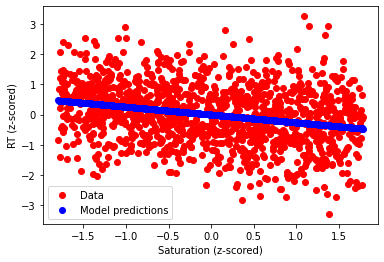
ax = plt.gca()
ax.scatter(df.saturation_std,df.RT_std,color='r',label='Data')
ax.scatter(df.saturation_std,
doubleStandardizedModel.predict(X=df.loc[:,['saturation_std']]),
color='b',label='Model predictions')
ax.set_xlabel("Saturation (z-scored)")
ax.set_ylabel("RT (z-scored)")
plt.legend()
plt.show()
plt.close()
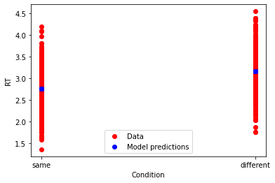
We can also fit a model to our categorical variables, such that we can see if there’s a difference in RT between the same and different conditions. To do so, we need to set up a dummy variable for our condition, then fit the linear model.
1
2
3
4
5
6
7
8
9
10
11
12
13
14
15
16
17
18
19
20
21
22
df['conditionDummy'], uniques = pd.factorize(df.condition)
print(uniques)
conditionModel = lm().fit(X=df.loc[:,['conditionDummy']],y=df.RT)


ax = plt.gca()

ax.scatter(df.conditionDummy,df.RT,color='r',label='Data')
ax.scatter(df.conditionDummy,
           conditionModel.predict(X=df.loc[:,['conditionDummy']]),
           color='b',label='Model predictions')
ax.set_xticks([0,1])
ax.set_xticklabels(list(uniques))
ax.set_xlabel("Condition")
ax.set_ylabel("RT")
plt.legend()
plt.show()
plt.close()

Index(['same', 'different'], dtype='object')
2.7520304353801066
[0.41476131]
If we want a library that does statistical testing and lets us specify some more complicated formulas (and then take care of the work that entails on the backend), we can use statsmodels! This lets us extend our linear models to the realm of interactions using some R-friendly syntax.
1
2
3
4
5
6
7
8
9
10
11
12
13
14
15
16
17
18
19
20
21
22
23
24
25
26
27
28
29
30
31
32
33
34
35
36
37
38
39
40
41
42
43
44
45
46
47
48
49
50
51
52
53
54
55
56
57
import statsmodels.api as sm
import statsmodels.formula.api as smf

results = smf.ols('RT ~ 1', data=df).fit() # original intercept model!!
print(results.summary())
results2 = smf.ols('RT ~ 1 + saturation',data=df).fit() # saturation model!!!
print(results2.summary())

                            OLS Regression Results
==============================================================================
Dep. Variable:                     RT   R-squared:                      -0.000
Model:                            OLS   Adj. R-squared:                 -0.000
Method:                 Least Squares   F-statistic:                       nan
Date:                Thu, 14 Sep 2023   Prob (F-statistic):                nan
Time:                        22:52:00   Log-Likelihood:                -872.93
No. Observations:                1250   AIC:                             1748.
Df Residuals:                    1249   BIC:                             1753.
Df Model:                           0
Covariance Type:            nonrobust
==============================================================================
                 coef    std err          t      P>|t|      [0.025      0.975]
------------------------------------------------------------------------------
Intercept      2.9594      0.014    214.998      0.000       2.932       2.986
==============================================================================
Omnibus:                        0.528   Durbin-Watson:                   2.303
Prob(Omnibus):                  0.768   Jarque-Bera (JB):                0.557
Skew:                          -0.049   Prob(JB):                        0.757
Kurtosis:                       2.969   Cond. No.                         1.00
==============================================================================

Notes:
[1] Standard Errors assume that the covariance matrix of the errors is correctly specified.
                            OLS Regression Results
==============================================================================
Dep. Variable:                     RT   R-squared:                       0.067
Model:                            OLS   Adj. R-squared:                  0.067
Method:                 Least Squares   F-statistic:                     90.17
Date:                Thu, 14 Sep 2023   Prob (F-statistic):           1.07e-20
Time:                        22:52:00   Log-Likelihood:                -829.33
No. Observations:                1250   AIC:                             1663.
Df Residuals:                    1248   BIC:                             1673.
Df Model:                           1
Covariance Type:            nonrobust
==============================================================================
                 coef    std err          t      P>|t|      [0.025      0.975]
------------------------------------------------------------------------------
Intercept      3.1889      0.028    115.595      0.000       3.135       3.243
saturation    -0.4547      0.048     -9.496      0.000      -0.549      -0.361
==============================================================================
Omnibus:                        0.502   Durbin-Watson:                   2.382
Prob(Omnibus):                  0.778   Jarque-Bera (JB):                0.431
Skew:                           0.041   Prob(JB):                        0.806
Kurtosis:                       3.040   Cond. No.                         4.58
==============================================================================

Notes:
[1] Standard Errors assume that the covariance matrix of the errors is correctly specified.
The benefit of doing things using statsmodels (in addition to the nice model description that we get out) is that we can also easily specify interaction models: things of the form
y = β0 + β1x1 + β2x2 + β3x1 * x2
1
2
3
4
5
6
7
8
9
10
11
12
13
14
15
16
17
18
19
20
21
22
23
24
25
26
27
28
29
30
results3 = smf.ols('RT ~ 1 + saturation*condition',data=df).fit() # interaction model!!!
print(results3.summary())

                            OLS Regression Results
==============================================================================
Dep. Variable:                     RT   R-squared:                       0.260
Model:                            OLS   Adj. R-squared:                  0.258
Method:                 Least Squares   F-statistic:                     145.8
Date:                Thu, 14 Sep 2023   Prob (F-statistic):           5.68e-81
Time:                        22:52:02   Log-Likelihood:                -684.89
No. Observations:                1250   AIC:                             1378.
Df Residuals:                    1246   BIC:                             1398.
Df Model:                           3
Covariance Type:            nonrobust
================================================================================================
                                   coef    std err          t      P>|t|      [0.025      0.975]
------------------------------------------------------------------------------------------------
Intercept                        3.3670      0.035     95.795      0.000       3.298       3.436
condition[T.same]               -0.3303      0.049     -6.711      0.000      -0.427      -0.234
saturation                      -0.3893      0.060     -6.480      0.000      -0.507      -0.271
saturation:condition[T.same]    -0.1856      0.085     -2.172      0.030      -0.353      -0.018
==============================================================================
Omnibus:                        1.395   Durbin-Watson:                   1.975
Prob(Omnibus):                  0.498   Jarque-Bera (JB):                1.294
Skew:                           0.038   Prob(JB):                        0.524
Kurtosis:                       3.138   Cond. No.                         12.0
==============================================================================

Notes:
[1] Standard Errors assume that the covariance matrix of the errors is correctly specified.
And that just about covers the basics of linear regression in Python! If you want more information on sklearn’s linear regression, you can check out sklearn’s documentation, and the same for statsmodels. For information about interpreting linear regression results, again: take a look at Kevin’s tutorial!