
Multilevel models: what, why, and how
Analyzing data with repeated observations for a particular participant, stimulus, or other group is one of the most common things you need to do in psychology & neuroscience, like most sciences. If you’ve ever done it, however, you’ll know that these repeated observations can cause serious methodological challenges. Despite (and perhaps because of) countless tutorial papers and statisticians yelling their diverse opinions out into the scientific literature, it can still be hard to know what to do when starting out.
Here we’re going to be discussing multilevel models (also confusingly known as mixed-effect models, linear mixed-effect regressions, or hierarchical models), which is in most cases the preferred way of analyzing data with repeated observations.
Regression refresher
Before we dive into multilevel models, it’ll be helpful to first have a reminder of the setup for a good old fashioned regression. Remember that in regression, we’re estimating an equation of the form
\[\begin{align*} y_n &\sim \mathcal{N}(\mu_n, \sigma) \\ \mu_n &= \beta X_n + \alpha \end{align*}\]which should look familiar if you’ve ever taken an algebra class. Here \(y\) is the outcome variable or the dependent variable, which is the thing we’re trying to predict. The subscript \(y_n\) identifies the n-th row of the data. The first line of this equation says that we want to model \(y\) as normally distributed with mean \(\mu_n\) and standard deviation \(\sigma\) (the ~ can be read as is distributed as).
How do we determine what the mean \(\mu_n\) should be? Using predictors!
\(X\) is a set of predictor variables or independent variables, which we
are using to predict \(\mu\). Again, the subscript \(X_n\) refers to the
n-th row of the data, so that each row has its own predictors and its
own mean. Then, \(\alpha\) is the intercept, which means that it is the
value of \(\mu\) when all of the \(X\)’s are set to 0. Finally,
\(\beta\) is a set of the slopes of each \(X\) on \(\mu\)- for every
increase in \(X_i\) by 1, the value of \(\mu\) increases by
\(\beta_i\) on average.
Let’s focus on a case where we have no predictors, and we just want to estimate the mean value of some variable. In particular, let’s say that we are recording a single rating from a bunch of different participants on …, and we want to know what the mean rating is. This simplifies our model to the following form:
\[\begin{align*} y_n &\sim \mathcal{N}(\alpha, \sigma) \\ \end{align*}\]If these equations are hurting your brain, it might help to visualize our model using the following diagram:
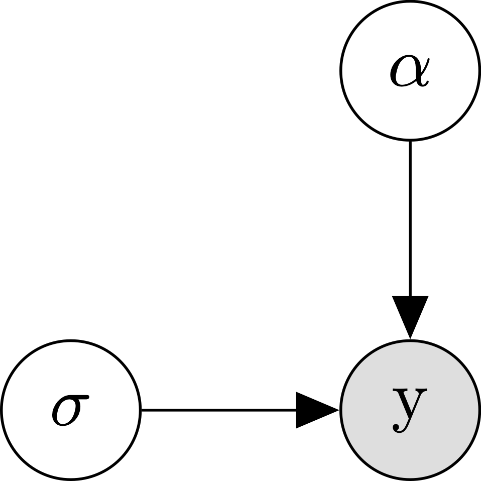
This graph says that our data \(y\) depends on two parameters, \(\alpha\) and \(\sigma\). Though the graph doesn’t exactly say how \(y\) depends on these parameters, our equation tells us that \(y\) follows a normal distribution with mean \(\alpha\) and standard deviation \(\sigma\).
We can simulate data from this model by specifying each of the parameters: without any predictors, we don’t have any \(\beta\)s, so the only parameters we need to specify are \(\alpha\) (the intercept) and \(\sigma\) (the residual standard deviation). For now, we can pick those values arbitrarily to see what kinds of things we can do by changing the parameters:
1
2
3
4
5
6
7
8
9
10
11
12
13
14
15
16
17
18
19
20
21
22
23
24
25
library(tidyverse)
library(lme4)
library(ggdist)

N_participants <- 500      ## number of data points to simulate
ALPHA <- c(-1, 0, 1)       ## mean of simulated data
SIGMA <- c(0.25, 0.5, 1)   ## SD of simulated data

## simulate datasets with different values of MU and SIGMA
d <- expand_grid(participant=as.factor(1:N_participants),
                 mu=ALPHA,
                 sigma=SIGMA) %>%
    mutate(y=rnorm(n(), mu, sigma))

## plot the simulated data
ggplot(d, aes(x=y)) +
    stat_slab() +
    scale_y_continuous(expand=c(0, 0)) +
    scale_fill_discrete(name='Participant') +
    facet_grid(mu ~ sigma, labeller=label_both) +
    theme_bw() +
    theme(axis.title.y=element_blank(),
          axis.text.y=element_blank(),
          axis.ticks.y=element_blank(),
          axis.line.y=element_blank())
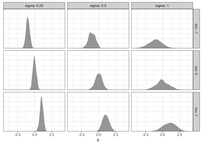
What patterns do you see? As \(\alpha\) increases, the average rating increases proportionally. In contrast, when \(\sigma\) increases, the average rating is the same, but the data become more spread out (i.e., they have a higher standard deviation).
Across the board, however, different participants tend to give different ratings. Since we’ve only collected a single rating per participant, it’s difficult to know whether that rating truly reflects their beliefs, or if that particular rating was an outlier for that particular individual. To understand things better at the participant-level, we need to collect many data points per participants.
Simulating three possible repeated measures datasets
Before we get into some different ways of analyzing repeated-measures data, it will be helpful to simulate three different ways that repeated measures data can look. Later, we can use these three datasets to test the performance of our different models.
When participants are completely similar
One possibility is that all of our participants will behave exactly the same- no matter which participants’ data we look at, it looks the same. This is the easiest to simulate, since it’s basically the same as simulating data from a single participant:
1
2
3
4
5
6
7
8
9
10
## simulate a dataset assuming equal ALPHA per participant
N_participants <- 5      ## number of participants to simulate
N_trials <- 500          ## number of data points per participant to simulate
ALPHA <- 0               ## mean of simulated data
SIGMA <- 0.2             ## SD of simulated data

d1 <- expand_grid(participant=as.factor(1:N_participants),
                  trial=as.factor(1:N_trials)) %>%
    mutate(y=rnorm(n(), ALPHA, SIGMA))
d1
1
2
3
4
5
6
7
8
9
10
11
12
13
14
## # A tibble: 2,500 × 3
##    participant trial       y
##    <fct>       <fct>   <dbl>
##  1 1           1     -0.173
##  2 1           2     -0.288
##  3 1           3     -0.105
##  4 1           4     -0.301
##  5 1           5     -0.0475
##  6 1           6     -0.0817
##  7 1           7     -0.0798
##  8 1           8      0.275
##  9 1           9      0.190
## 10 1           10     0.224
## # ℹ 2,490 more rows
Here we’re using the expand_grid function to generate every possible
combination of participant and trial numbers, then we’re using rnorm
to generate data from a normal distribution. Let’s plot our data to make
sure it looks right:
1
2
3
4
5
6
7
8
9
10
## plot the simulated data
ggplot(d1, aes(x=y, fill=participant)) +
    stat_slab(alpha=.25) +
    scale_y_continuous(expand=c(0, 0)) +
    scale_fill_discrete(name='Participant') +
    theme_bw() +
    theme(axis.title.y=element_blank(),
          axis.text.y=element_blank(),
          axis.ticks.y=element_blank(),
          axis.line.y=element_blank())
Sweet- just like we wanted, all of the participants look about the same.
When participants are completely different
Another possibility is that our participants are completely different
from each other. Let’s assume that each participant has an individual
mean that is uniformly spread across a pretty wide range from -1 to
1. Here we’ll use the seq function to make a mean for each
participant, and then we can simulate the data for each participant just
like before:
1
2
3
4
5
6
ALPHA_participant2 <- seq(-1, 1, length.out=N_participants)

d2 <- expand_grid(participant=as.factor(1:N_participants),
                  trial=as.factor(1:N_trials)) %>%
    mutate(y=rnorm(n(), ALPHA_participant2[participant], SIGMA))
d2
1
2
3
4
5
6
7
8
9
10
11
12
13
14
## # A tibble: 2,500 × 3
##    participant trial      y
##    <fct>       <fct>  <dbl>
##  1 1           1     -0.928
##  2 1           2     -0.977
##  3 1           3     -1.03
##  4 1           4     -1.29
##  5 1           5     -0.844
##  6 1           6     -0.730
##  7 1           7     -1.15
##  8 1           8     -0.791
##  9 1           9     -0.998
## 10 1           10    -1.01
## # ℹ 2,490 more rows
To make sure this looks right, we can plot the data as before:
1
2
3
4
5
6
7
8
9
ggplot(d2, aes(x=y, fill=participant)) +
    stat_slab(alpha=.25) +
    scale_y_continuous(expand=c(0, 0)) +
    scale_fill_discrete(name='Participant') +
    theme_bw() +
    theme(axis.title.y=element_blank(),
          axis.text.y=element_blank(),
          axis.ticks.y=element_blank(),
          axis.line.y=element_blank())
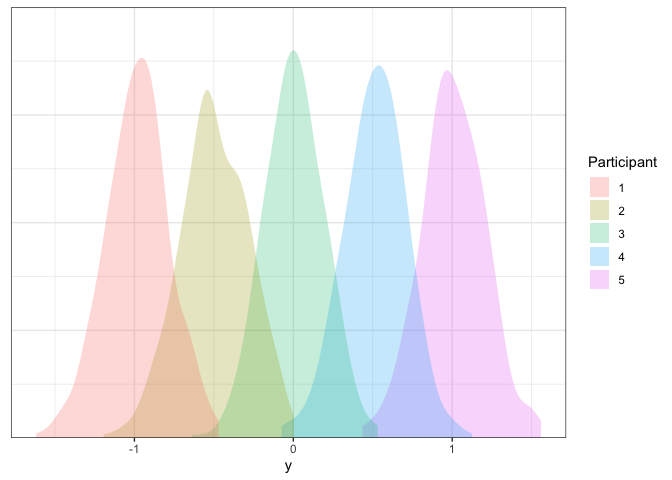
Looks good!
When some participants are outliers
Finally, we can imagine a scenario where most of our participants are
similar (or even the same), but there are potentially some outliers that
consistently respond with extreme ratings. For this dataset, we’ll
assume that all of our participants have a mean rating of 0, but
there’s a single participant with a mean of 2. As before, we’ll define
a vector containing the mean for each participant, and we’ll use those
means to simulate our data:
1
2
3
4
5
ALPHA_participant3 <- c(rep(0, times=N_participants-1), 2)

d3 <- expand_grid(participant=as.factor(1:N_participants),
                  trial=as.factor(1:N_trials)) %>%
    mutate(y=rnorm(n(), ALPHA_participant3[participant], SIGMA))
Let’s plot our data one more time to make sure it’s good:
1
2
3
4
5
6
7
8
9
ggplot(d3, aes(x=y, fill=participant)) +
    stat_slab(alpha=.25) +
    scale_y_continuous(expand=c(0, 0)) +
    scale_fill_discrete(name='Participant') +
    theme_bw() +
    theme(axis.title.y=element_blank(),
          axis.text.y=element_blank(),
          axis.ticks.y=element_blank(),
          axis.line.y=element_blank())
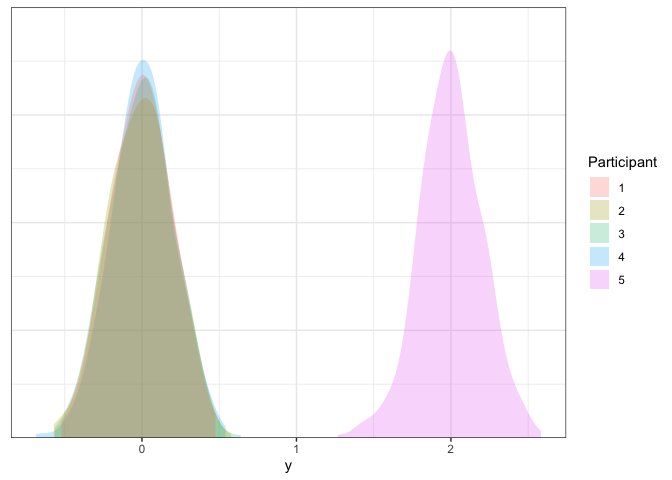
Good stuff! Now that we have some repeated measures datasets in hand, we can explore different ways of analyzing these data.
The naive approach (complete pooling)
If you have many ratings per participant, one way to analyze this data is ignore the fact that each participants could be different and to assume a single distribution from which ratings are drawn. Another way to think about this is that you’re pretending that each response comes from a completely different individual. That is, we can use the same regression model we had before:
\[\begin{align*} y_n &\sim \mathcal{N}(\alpha, \sigma) \\ \end{align*}\]
So, even though in reality it might be that different participants have different \(\alpha\)s, we’re going to pretend that \(\alpha\) is the same for everyone. As a result, we call this approach complete pooling, since we are pooling all the data from different participants together to estimate just one single \(\alpha\).
Estimating the complete pooling model
Given the constraint that different participants have the same mean rating, you can likely predict when this model will work fine and when it will lead you astray. Let’s try it out on our three different datasets:
When participants are similar
To start simple, let’s analyze the dataset we simulated above where the
assumption that participants are similar holds. We’re going to use the
lm function, which fits any standard regression:
1
2
m1.complete <- lm(y ~ 1, data=d1)
summary(m1.complete)
1
2
3
4
5
6
7
8
9
10
11
12
13
14
15
##
## Call:
## lm(formula = y ~ 1, data = d1)
##
## Residuals:
##      Min       1Q   Median       3Q      Max
## -0.82256 -0.13351  0.00126  0.13386  0.58121
##
## Coefficients:
##              Estimate Std. Error t value Pr(>|t|)
## (Intercept) -0.008256   0.003910  -2.112   0.0348 *
## ---
## Signif. codes:  0 '***' 0.001 '**' 0.01 '*' 0.05 '.' 0.1 ' ' 1
##
## Residual standard error: 0.1955 on 2499 degrees of freedom
This summary gives us two important pieces of information. First, under
coefficients, the (Intercept) is our \(\alpha\) parameter. The
estimate is close to our true value of 0, and the high p-value says
that it is not significantly different from 0 (for more information on
p-values, check out my earlier post
here). Second, the last
line says that our residual standard error (\(\sigma\) in our equation
above) is close to the true value of 0.2. Overall, when different
participants are indeed similar, this model gives us very good parameter
estimates!
Just to be 100% sure that this is the case, we can simulate data from
our estimated model to check that it looks like our actual data. We call
this simulated data \(\hat{y}\) or y_hat, to contrast it with the real
data \(y\). We can do this using the simulate function:
1
2
3
4
5
6
7
8
9
10
11
12
13
d1 <- d1 %>% mutate(y_hat_complete=simulate(m1.complete)$sim_1)

d1 %>% pivot_longer(y:y_hat_complete) %>%
    ggplot(aes(x=value, fill=participant)) +
    stat_slab(alpha=.25) +
    scale_y_continuous(expand=c(0, 0)) +
    scale_fill_discrete(name='Participant') +
    facet_grid(name ~ .) +
    theme_bw() +
    theme(axis.title.y=element_blank(),
          axis.text.y=element_blank(),
          axis.ticks.y=element_blank(),
          axis.line.y=element_blank())
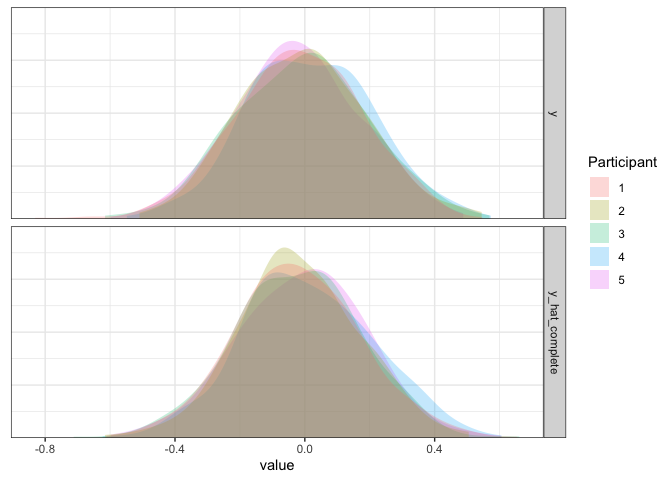
Confirming our intuitions above, the data simulated from our fitted model looks a lot like “actual” data, which means it is doing pretty good! Of course, however, it isn’t always the case that different participants will have the same average rating. For example, different participants might be better or worse at a task, more optimistic/pessimistic, or just have different opinions from each other. We can focus on two examples where this might be the case.
When participants are different
Next, let’s look at our second dataset where each participant has a reliable mean rating, but each participants’ mean ratings are completely different from each other. What happens if we fit our naive complete pooling model?
1
2
m2.complete <- lm(y ~ 1, data=d2)
summary(m2.complete)
1
2
3
4
5
6
7
8
9
10
11
12
13
##
## Call:
## lm(formula = y ~ 1, data = d2)
##
## Residuals:
##      Min       1Q   Median       3Q      Max
## -1.62799 -0.62519 -0.00818  0.61986  1.54859
##
## Coefficients:
##             Estimate Std. Error t value Pr(>|t|)
## (Intercept) 0.009834   0.014674    0.67    0.503
##
## Residual standard error: 0.7337 on 2499 degrees of freedom
Overall, the model fit looks very similar! There is one interesting
change, however: the estimated residual standard error is now off!
Rather than being close to the true value of \(\sigma\) = .2, it is
estimated to be above .7. Why is this? To get a better idea, let’s
simulate our data again from our fitted model:
1
2
3
4
5
6
7
8
9
10
11
12
13
d2 <- d2 %>% mutate(y_hat_complete=simulate(m2.complete)$sim_1)

d2 %>% pivot_longer(y:y_hat_complete) %>%
    ggplot(aes(x=value, fill=participant)) +
    stat_slab(alpha=.25) +
    scale_y_continuous(expand=c(0, 0)) +
    scale_fill_discrete(name='Participant') +
    facet_grid(name ~ .) +
    theme_bw() +
    theme(axis.title.y=element_blank(),
          axis.text.y=element_blank(),
          axis.ticks.y=element_blank(),
          axis.line.y=element_blank())
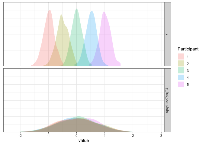
Remember that our model assumes that participants all have the same mean? In the case where participants are different, our model has only one way to account for ratings that are far away from the mean: by making the standard deviation large. So, rather than having a bunch of narrow distributions that are spread apart, we have one big distribution that’s wide enough to account for everything. Not ideal, but not the worst: we might not have a good idea of how participants differ, but at least our estimate of the mean is good enough.
With outliers
Finally, let’s look at our dataset where most participants are the same but there’s one outlier:
1
2
m3.complete <- lm(y ~ 1, data=d3)
summary(m3.complete)
1
2
3
4
5
6
7
8
9
10
11
12
13
14
15
##
## Call:
## lm(formula = y ~ 1, data = d3)
##
## Residuals:
##      Min       1Q   Median       3Q      Max
## -1.08196 -0.50005 -0.33158 -0.08697  2.18594
##
## Coefficients:
##             Estimate Std. Error t value Pr(>|t|)
## (Intercept)  0.39689    0.01651   24.03   <2e-16 ***
## ---
## Signif. codes:  0 '***' 0.001 '**' 0.01 '*' 0.05 '.' 0.1 ' ' 1
##
## Residual standard error: 0.8257 on 2499 degrees of freedom
Well, that’s not good. Not only is the residual standard deviation still
high, but the intercept is now .4 (significantly above 0)! To get a
better idea of what’s going on, let’s simulate data from our fitted
model:
1
2
3
4
5
6
7
8
9
10
11
12
13
d3 <- d3 %>% mutate(y_hat_complete=simulate(m3.complete)$sim_1)

d3 %>% pivot_longer(y:y_hat_complete) %>%
    ggplot(aes(x=value, fill=participant)) +
    stat_slab(alpha=.25) +
    scale_y_continuous(expand=c(0, 0)) +
    scale_fill_discrete(name='Participant') +
    facet_grid(name ~ .) +
    theme_bw() +
    theme(axis.title.y=element_blank(),
          axis.text.y=element_blank(),
          axis.ticks.y=element_blank(),
          axis.line.y=element_blank())
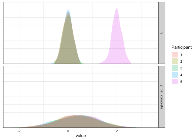
As we can see, this model is not good. Not only is the simulated data way too widely dispersed, but the mean is biased by the single outlier participant. So, if there is a potential for outliers, this approach cannot handle them effectively.
Complete pooling summary
Overall, the complete pooling model doesn’t seem to be ideal. When participants are very similar, the model does fine. But, the more participants differ, the worse this model will perform: it’ll be biased by outliers, and it’ll overestimate the residual standard deviation. This might not sound like a serious problem, but it is: results that should be significant might turn out non-significant, and results that shouldn’t be significant might appear to be significant.
Some more nuance (no pooling)
Well if lumping all of our participants’ data together didn’t work, what else can we do? The next obvious choice is to analyze each participant separately. We’re going to call this the no pooling approach, since we’re not going to assume any similarity between participants- each participants’ data will go into a separate pool. Formally, we are just replacing our single \(\alpha\) parameter with a separate \(\alpha_{p[n]}\) parameter per participant, where \(p[n]\) indexes the participant for trial \(n\):
\[\begin{align*} y_n &\sim \mathcal{N}(\alpha_{p[n]}, \sigma) \\ \end{align*}\]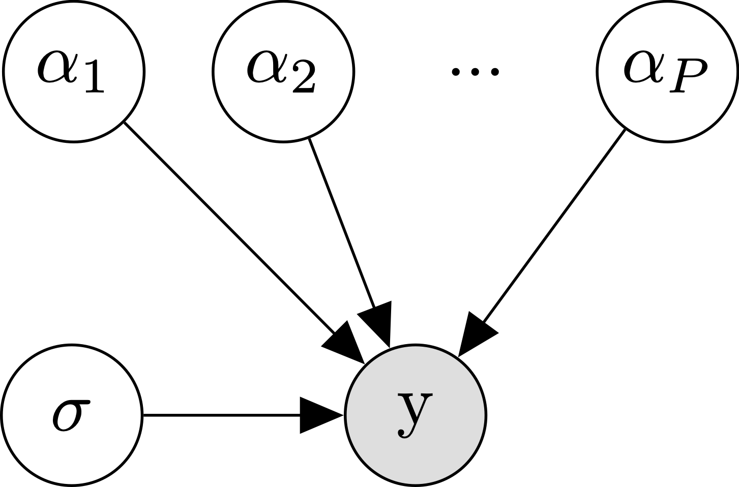
The diagram makes it clear that where we used to just have one \(\alpha\), we now have to independently estimate \(P\) different \(\alpha\)s.
Estimating the no pooling model
As with the complete pooling model, let’s try the no pooling model out on our three datasets.
When participants are similar
To estimate the no-pooling model, we’re going to make use of a neat
statistical trick. Instead of literally fitting a separate model per
participant, we can instead add participant ID as a predictor variable
to our model. This is much easier, and turns out to be essentially the
same thing. We’ll make use of a special formula syntax
y ~ 0 + participant, which means that our model includes no intercept
(hence the 0), but instead a coefficient for each participant (hence
the participant).
1
2
m1.no <- lm(y ~ 0 + participant, data=d1)
summary(m1.no)
1
2
3
4
5
6
7
8
9
10
11
12
13
14
15
16
17
18
19
20
21
##
## Call:
## lm(formula = y ~ 0 + participant, data = d1)
##
## Residuals:
##      Min       1Q   Median       3Q      Max
## -0.81198 -0.13546  0.00079  0.13285  0.57696
##
## Coefficients:
##               Estimate Std. Error t value Pr(>|t|)
## participant1 -0.018839   0.008728  -2.158   0.0310 *
## participant2 -0.006732   0.008728  -0.771   0.4406
## participant3 -0.007990   0.008728  -0.915   0.3600
## participant4  0.016055   0.008728   1.840   0.0660 .
## participant5 -0.023773   0.008728  -2.724   0.0065 **
## ---
## Signif. codes:  0 '***' 0.001 '**' 0.01 '*' 0.05 '.' 0.1 ' ' 1
##
## Residual standard error: 0.1952 on 2495 degrees of freedom
## Multiple R-squared:  0.006726,   Adjusted R-squared:  0.004735
## F-statistic: 3.379 on 5 and 2495 DF,  p-value: 0.004798
The summary looks a bit more complicated (one coefficient per
participant), but the no-pooling model does OK when participants are
similar. All of the participants are close to their true values of 0
(though some may be significantly different from 0 due to noise).
Likewise, the residual standard error is close to its true value of
.2. As before, we can simulate data from the fitted model to confirm:
1
2
3
4
5
6
7
8
9
10
11
12
13
d1 <- d1 %>% mutate(y_hat_no=simulate(m1.no)$sim_1)

d1 %>% pivot_longer(c(y, y_hat_no)) %>%
    ggplot(aes(x=value, fill=participant)) +
    stat_slab(alpha=.25) +
    scale_y_continuous(expand=c(0, 0)) +
    scale_fill_discrete(name='Participant') +
    facet_grid(name ~ .) +
    theme_bw() +
    theme(axis.title.y=element_blank(),
          axis.text.y=element_blank(),
          axis.ticks.y=element_blank(),
          axis.line.y=element_blank())
As expected, the simulated data from this model match the true data pretty well.
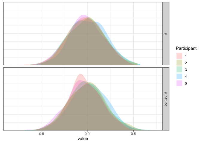
When participants are different
Next, let’s try it out when participants are completely different:
1
2
m2.no <- lm(y ~ 0 + participant, data=d2)
summary(m2.no)
1
2
3
4
5
6
7
8
9
10
11
12
13
14
15
16
17
18
19
20
21
##
## Call:
## lm(formula = y ~ 0 + participant, data = d2)
##
## Residuals:
##      Min       1Q   Median       3Q      Max
## -0.69596 -0.12869 -0.00246  0.13656  0.60929
##
## Coefficients:
##               Estimate Std. Error  t value Pr(>|t|)
## participant1 -0.983044   0.008862 -110.931   <2e-16 ***
## participant2 -0.497634   0.008862  -56.155   <2e-16 ***
## participant3  0.006842   0.008862    0.772     0.44
## participant4  0.515181   0.008862   58.135   <2e-16 ***
## participant5  1.007827   0.008862  113.727   <2e-16 ***
## ---
## Signif. codes:  0 '***' 0.001 '**' 0.01 '*' 0.05 '.' 0.1 ' ' 1
##
## Residual standard error: 0.1982 on 2495 degrees of freedom
## Multiple R-squared:  0.9272, Adjusted R-squared:  0.927
## F-statistic:  6355 on 5 and 2495 DF,  p-value: < 2.2e-16
Gee, I’m seeing stars! All of the participants with means away from zero are correctly idendified as being significantly different from zero. Our residual standard error is also looking just fine! Again, we can simulate and plot to double check:
1
2
3
4
5
6
7
8
9
10
11
12
13
d2 <- d2 %>% mutate(y_hat_no=simulate(m2.no)$sim_1)

d2 %>% pivot_longer(c(y, y_hat_no)) %>%
    ggplot(aes(x=value, fill=participant)) +
    stat_slab(alpha=.25) +
    scale_y_continuous(expand=c(0, 0)) +
    scale_fill_discrete(name='Participant') +
    facet_grid(name ~ .) +
    theme_bw() +
    theme(axis.title.y=element_blank(),
          axis.text.y=element_blank(),
          axis.ticks.y=element_blank(),
          axis.line.y=element_blank())

Looks great to me!
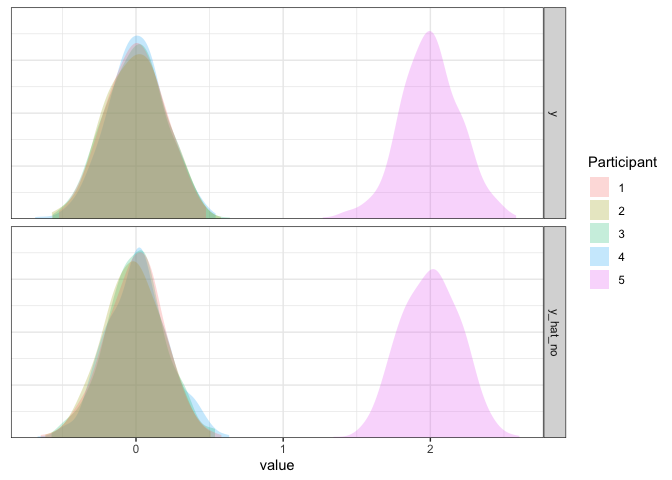
When there are outliers
Finally, we can try the no pooling approach when there are outliers:
1
2
m3.no <- lm(y ~ 0 + participant, data=d3)
summary(m3.no)
1
2
3
4
5
6
7
8
9
10
11
12
13
14
15
16
17
18
19
20
21
##
## Call:
## lm(formula = y ~ 0 + participant, data = d3)
##
## Residuals:
##      Min       1Q   Median       3Q      Max
## -0.72958 -0.13704  0.00044  0.13353  0.64443
##
## Coefficients:
##               Estimate Std. Error t value Pr(>|t|)
## participant1 -0.005807   0.008988  -0.646    0.518
## participant2 -0.007476   0.008988  -0.832    0.406
## participant3 -0.006271   0.008988  -0.698    0.485
## participant4  0.005687   0.008988   0.633    0.527
## participant5  1.998293   0.008988 222.318   <2e-16 ***
## ---
## Signif. codes:  0 '***' 0.001 '**' 0.01 '*' 0.05 '.' 0.1 ' ' 1
##
## Residual standard error: 0.201 on 2495 degrees of freedom
## Multiple R-squared:  0.9519, Adjusted R-squared:  0.9519
## F-statistic:  9885 on 5 and 2495 DF,  p-value: < 2.2e-16
Everything is still looking good! All participants are estimated to be
close to 0, participant 5 is correctly identified as having a mean
greater than 0, and the residual standard deviation is close to the
true value of .2. We can simulate and plot data one more time to be
sure:
1
2
3
4
5
6
7
8
9
10
11
12
13
d3 <- d3 %>% mutate(y_hat_no=simulate(m3.no)$sim_1)

d3 %>% pivot_longer(c(y, y_hat_no)) %>%
    ggplot(aes(x=value, fill=participant)) +
    stat_slab(alpha=.25) +
    scale_y_continuous(expand=c(0, 0)) +
    scale_fill_discrete(name='Participant') +
    facet_grid(name ~ .) +
    theme_bw() +
    theme(axis.title.y=element_blank(),
          axis.text.y=element_blank(),
          axis.ticks.y=element_blank(),
          axis.line.y=element_blank())
No pooling summary
From what we’ve seen here, the no pooling approach looks great: in each case, it correctly estimates the mean for each participant and correctly estimates the residual standard deviation. So, what could be missing (take a minute to think this through before reading on)?
The answer is that the no pooling approach is very data hungry, to the point that statistical power usually becomes a huge issue. If you think about what the no pooling approach does, this should make sense: to have the same statistical power to estimate a single participants’ effect that you would have to estimate a population-level mean in a between-participant design, you need as many data points per participant as you would normally need for the whole experiment!
This statistical power issue causes problems in two ways. First, it
might be difficult to detect a true effect as significant without a
massive amount of data. Second, you are more prone to ending up with a
significant effect even when the true effect is 0.
P.S. Another minor issue that people sometimes complain about is that
interpreting estimates from the no pooling approach is “complicated.”
But it’s actually very easy to do! The model summary gives you means per
participant, but you can use packages like emmeans to get the estimate
of the grand mean from your model. For example,
1
2
library(emmeans)
emmeans(m3.no, ~ 1)
1
2
3
4
5
##  1       emmean      SE   df lower.CL upper.CL
##  overall  0.397 0.00402 2495    0.389    0.405
##
## Results are averaged over the levels of: participant
## Confidence level used: 0.95
The goldilocks zone (partial pooling)
In the case where you don’t have a massive amount of data per participant (which, let’s be honest, is always), how can we allow our estimates of participant means to differ? The answer is that we can assume that even if participant means aren’t all the same, they should all be drawn from the same distribution. In particular, we’re going to assume that participant means follow a normal distribution where the mean is equal to the grand mean and the standard deviation is equal to the between-participant variability in mean rating. Technically speaking you could use any distribution you want here, but the normal distribution is nice, interpretable, efficient, and will work in most cases.
Formally speaking, we now have this model:
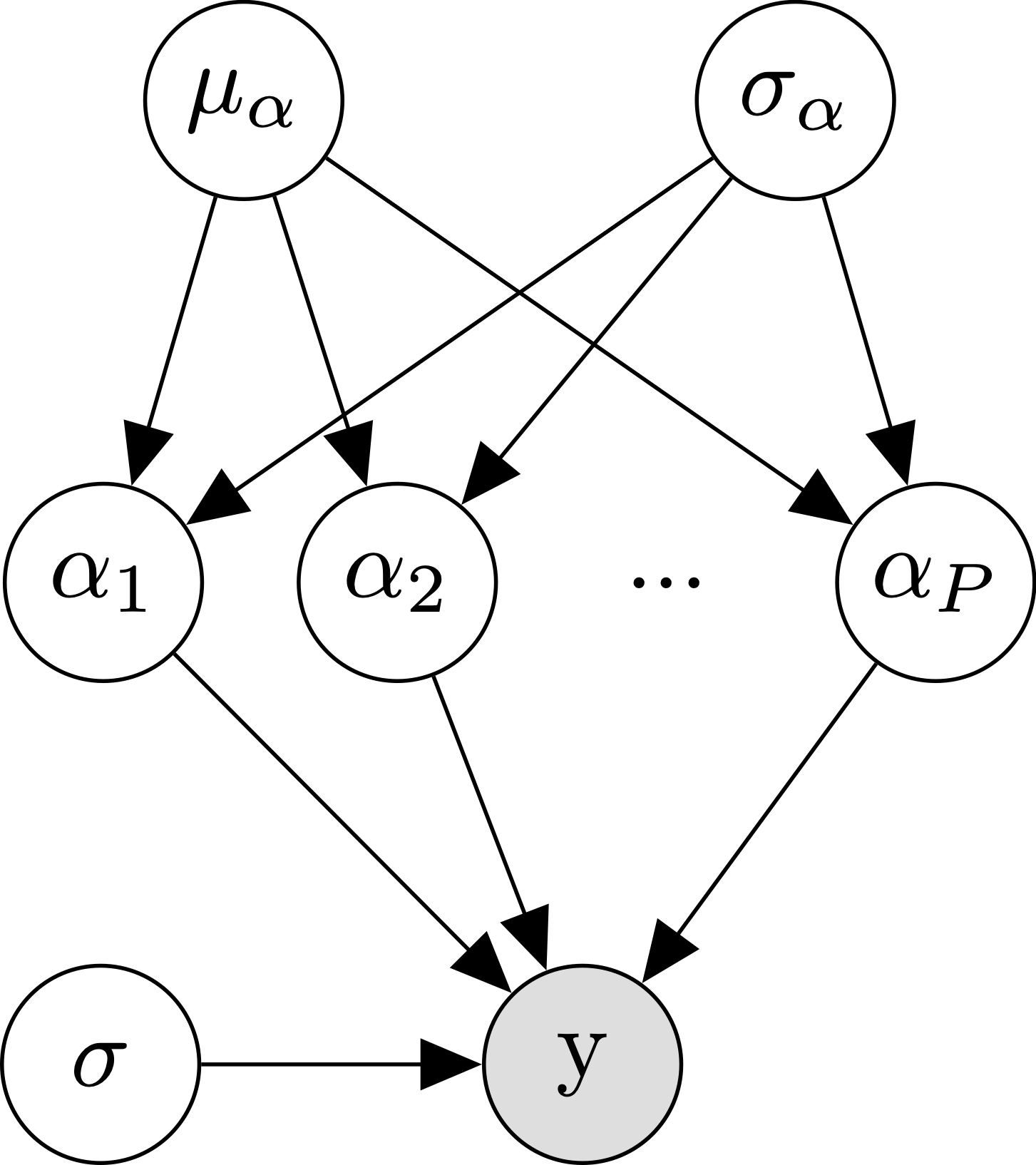
\[\begin{align*} y_n &\sim \mathcal{N}(\alpha_{p[n]}, \sigma) \\ \alpha_{p} &\sim \mathcal{N}(\mu_\alpha, \sigma_\alpha) \end{align*}\]
And here we have a multilevel model! We call it multilevel, since now our alpha parameters are being drawn from their own distribution, and the ratings are drawn using those random means. Hopefully the diagram makes this clear: where we used to just have one fixed \(\alpha\), we now have a bunch of randomly drawn \(\alpha\)s with mean \(\mu_\alpha\) and standard deviation \(\sigma_alpha\). This model is also referred to as a partial pooling model, since it is a happy medium between the complete pooling model (where everyone is the same) and the no pooling model (where everyone can be arbitrarily different).
Before we fit this model, we can simulate some data from it to get a feel for what is going on. We do this by starting from the bottom of the equations above, and working our way up (i.e., first simulating a mean per participant, then simulating the ratings):
1
2
3
4
5
6
7
8
SIGMA_MU <- .5    ## between-participant standard deviation

d4 <- expand_grid(participant=1:N_participants, trial=1:N_trials) %>%
    group_by(participant) %>%
    mutate(alpha=rnorm(1, ALPHA, SIGMA_MU)) %>%   ## simulate a partipant-level mean
    ungroup() %>%
    mutate(y=rnorm(n(), alpha, SIGMA))         ## simulate the ratings
d4
1
2
3
4
5
6
7
8
9
10
11
12
13
14
## # A tibble: 2,500 × 4
##    participant trial  alpha      y
##          <int> <int>  <dbl>  <dbl>
##  1           1     1 -0.743 -0.885
##  2           1     2 -0.743 -0.693
##  3           1     3 -0.743 -0.537
##  4           1     4 -0.743 -0.859
##  5           1     5 -0.743 -0.540
##  6           1     6 -0.743 -0.467
##  7           1     7 -0.743 -0.692
##  8           1     8 -0.743 -0.531
##  9           1     9 -0.743 -0.580
## 10           1    10 -0.743 -0.672
## # ℹ 2,490 more rows
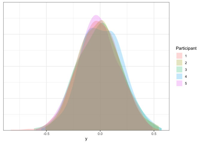
Looks promising! Let’s plot our data to see how it looks. Here I’ll plot the participant-level data as before:
1
2
3
4
5
6
7
8
9
10
ggplot(d4, aes(x=y, group=participant, fill=factor(participant))) +
    stat_slab(slab_alpha=0.25) +
    scale_x_continuous('Rating') +
    scale_y_continuous(expand=c(0, 0)) +
    scale_fill_discrete(name='Participant') +
    theme_ggdist() +
    theme(axis.title.y=element_blank(),
          axis.text.y=element_blank(),
          axis.ticks.y=element_blank(),
          axis.line.y=element_blank())
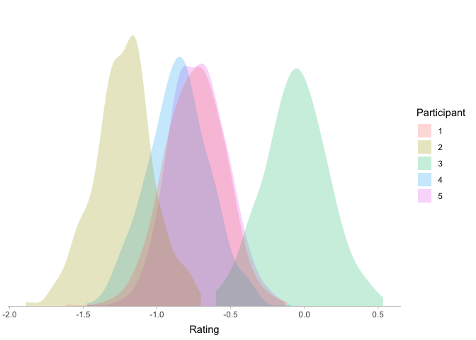
Looks like a happy medium! Our participants now differ from each other, but now the differences between participants are not arbitrary: most participants will be fairly similar, with some variation around the grand mean.
Estimating the partial pooling model
With this understanding of our model, we can test it on our three datasets as before.
When participants are similar
To estimate the partial pooling model, we can use the lmer function
(standing for linear mixed-effects regression) from the package
lme4. This works the same as lm, except now we can also define
participant-level parameters by adding the term (1 | participant) to
our model formula. You can interpret this as “a single intercept per
participant,” following a normal distribution:
1
2
m1.partial <- lmer(y ~ 1 + (1 | participant), data=d1)
summary(m1.partial)
1
2
3
4
5
6
7
8
9
10
11
12
13
14
15
16
17
18
19
## Linear mixed model fit by REML ['lmerMod']
## Formula: y ~ 1 + (1 | participant)
##    Data: d1
##
## REML criterion at convergence: -1062.1
##
## Scaled residuals:
##     Min      1Q  Median      3Q     Max
## -4.1779 -0.6894  0.0016  0.6806  2.9567
##
## Random effects:
##  Groups      Name        Variance  Std.Dev.
##  participant (Intercept) 0.0001604 0.01266
##  Residual                0.0380894 0.19517
## Number of obs: 2500, groups:  participant, 5
##
## Fixed effects:
##              Estimate Std. Error t value
## (Intercept) -0.008256   0.006878    -1.2
The summary looks still more complicated, but the partial pooling model
does well when participants are similar! Under the Fixed effects
(meaning averaged over participants) section, we can see that the
intercept is correctly identified as close to 0. Now we also get a new
section labeled Random effects, which describes our participant-level
parameters. The first line says that the variance in participant-level
means is 0, which is correct! Note that this is why we get the warning
about a singular fit: here lmer is trying to tell you that you don’t
need to model participant-level means if they are all the same. The
second line tells us that the residual standard deviation is close to
the true value of .2, which is also good! Again, we can simulate data
from the fitted model to confirm:
1
2
3
4
5
6
7
8
9
10
11
12
13
d1 <- d1 %>% mutate(y_hat_partial=simulate(m1.partial)$sim_1)

d1 %>% pivot_longer(c(y, y_hat_partial)) %>%
    ggplot(aes(x=value, fill=participant)) +
    stat_slab(alpha=.25) +
    scale_y_continuous(expand=c(0, 0)) +
    scale_fill_discrete(name='Participant') +
    facet_grid(name ~ .) +
    theme_bw() +
    theme(axis.title.y=element_blank(),
          axis.text.y=element_blank(),
          axis.ticks.y=element_blank(),
          axis.line.y=element_blank())
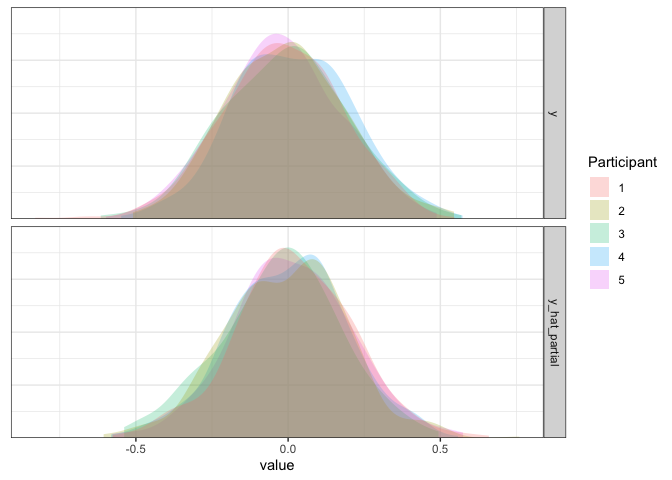
As expected, the simulated data from this model match the true data pretty well.
When participants are different
Next, let’s try it out when participants are completely different:
1
2
m2.partial <- lmer(y ~ 1 + (1 | participant), data=d2)
summary(m2.partial)
1
2
3
4
5
6
7
8
9
10
11
12
13
14
15
16
17
18
19
## Linear mixed model fit by REML ['lmerMod']
## Formula: y ~ 1 + (1 | participant)
##    Data: d2
##
## REML criterion at convergence: -954.7
##
## Scaled residuals:
##     Min      1Q  Median      3Q     Max
## -3.5125 -0.6492 -0.0121  0.6888  3.0751
##
## Random effects:
##  Groups      Name        Variance Std.Dev.
##  participant (Intercept) 0.62360  0.7897
##  Residual                0.03927  0.1982
## Number of obs: 2500, groups:  participant, 5
##
## Fixed effects:
##             Estimate Std. Error t value
## (Intercept) 0.009834   0.353179   0.028
Good stuff: the mean is correctly identified as near 0, and the
residual SD is close to .2. Furthermore, we now see that participants
differ with a standard deviation of about .8. Let’s simulate from the
fitted model to be sure this is right:
1
2
3
4
5
6
7
8
9
10
11
12
13
d2 <- d2 %>% mutate(y_hat_partial=simulate(m2.partial)$sim_1)

d2 %>% pivot_longer(c(y, y_hat_partial)) %>%
    ggplot(aes(x=value, fill=participant)) +
    stat_slab(alpha=.25) +
    scale_y_continuous(expand=c(0, 0)) +
    scale_fill_discrete(name='Participant') +
    facet_grid(name ~ .) +
    theme_bw() +
    theme(axis.title.y=element_blank(),
          axis.text.y=element_blank(),
          axis.ticks.y=element_blank(),
          axis.line.y=element_blank())
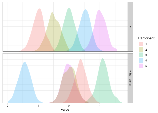
What’s going on here? The variation between participants seems about
right, but for some reason our participants aren’t lining up. It turns
out that the default for simulate.merMod is to ignore participant
labels and to simulate new participants instead. We can override this by
adding the argument re.form=NULL, which will use our actual
participant-level estimates:
1
2
3
4
5
6
7
8
9
10
11
12
13
d2 <- d2 %>% mutate(y_hat_partial=simulate(m2.partial, re.form=NULL)$sim_1)

d2 %>% pivot_longer(c(y, y_hat_partial)) %>%
    ggplot(aes(x=value, fill=participant)) +
    stat_slab(alpha=.25) +
    scale_y_continuous(expand=c(0, 0)) +
    scale_fill_discrete(name='Participant') +
    facet_grid(name ~ .) +
    theme_bw() +
    theme(axis.title.y=element_blank(),
          axis.text.y=element_blank(),
          axis.ticks.y=element_blank(),
          axis.line.y=element_blank())
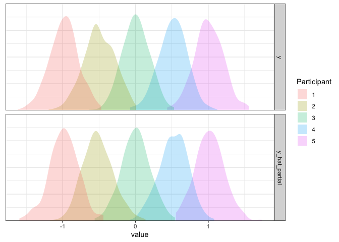
Now it’s looking good!
When there are outliers
Finally, we can try the partial pooling approach when there are outliers:
1
2
m3.partial <- lmer(y ~ 1 + (1 | participant), data=d3)
summary(m3.partial)
1
2
3
4
5
6
7
8
9
10
11
12
13
14
15
16
17
18
19
## Linear mixed model fit by REML ['lmerMod']
## Formula: y ~ 1 + (1 | participant)
##    Data: d3
##
## REML criterion at convergence: -882.9
##
## Scaled residuals:
##     Min      1Q  Median      3Q     Max
## -3.6292 -0.6820  0.0021  0.6641  3.2061
##
## Random effects:
##  Groups      Name        Variance Std.Dev.
##  participant (Intercept) 0.8014   0.8952
##  Residual                0.0404   0.2010
## Number of obs: 2500, groups:  participant, 5
##
## Fixed effects:
##             Estimate Std. Error t value
## (Intercept)   0.3969     0.4004   0.991
Again, looks good: the intercept and residual SD are correctly
estimated, and we have a new participant-level SD of .9. We can
simulate and plot data one more time to be sure:
1
2
3
4
5
6
7
8
9
10
11
12
13
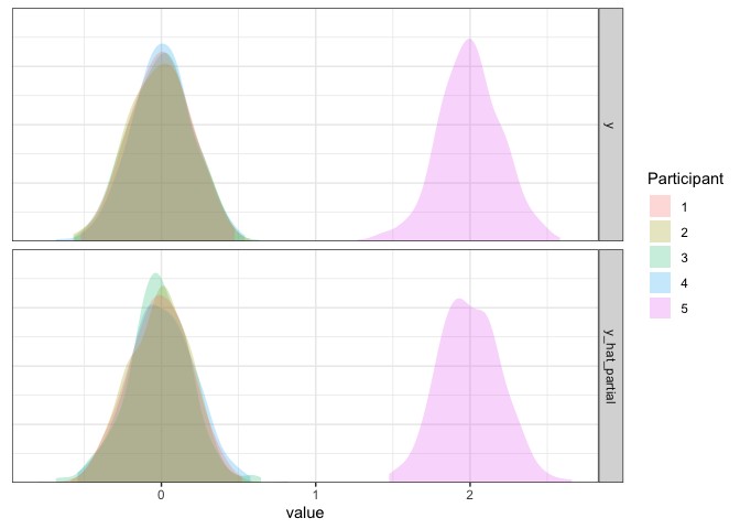
d3 <- d3 %>% mutate(y_hat_partial=simulate(m3.partial, re.form=NULL)$sim_1)
d3 %>% pivot_longer(c(y, y_hat_partial)) %>%
ggplot(aes(x=value, fill=participant)) +
stat_slab(alpha=.25) +
scale_y_continuous(expand=c(0, 0)) +
scale_fill_discrete(name='Participant') +
facet_grid(name ~ .) +
theme_bw() +
theme(axis.title.y=element_blank(),
axis.text.y=element_blank(),
axis.ticks.y=element_blank(),
axis.line.y=element_blank())
Partial pooling model summary
With our three datasets we’ve seen that the partial pooling model does as well as the no pooling model in recovering participant-level estimates of the mean. It also allows us to simulate new participants, which can help a TON when trying to run a power analysis via simulation (more on that here). But if that’s the only difference, why should we use the partial pooling model over the no pooling model?
Going back to something I said earlier, the no pooling model is data
hungry. In contrast, the partial pooling model will work well even if
data is sparse, as long as you have more than a few data points per
participant. To make this clear, we can fit our model to a subset of our
outlier dataset, using only 2 trials per participant instead of 500:
1
2
3
4
d4 <- d3 %>% group_by(participant) %>% sample_n(2)

m4 <- lmer(y ~ 1 + (1 | participant), d4)
summary(m4)
1
2
3
4
5
6
7
8
9
10
11
12
13
14
15
16
17
18
19
## Linear mixed model fit by REML ['lmerMod']
## Formula: y ~ 1 + (1 | participant)
##    Data: d4
##
## REML criterion at convergence: 10.5
##
## Scaled residuals:
##      Min       1Q   Median       3Q      Max
## -1.45172 -0.34703 -0.03004  0.31032  1.38088
##
## Random effects:
##  Groups      Name        Variance Std.Dev.
##  participant (Intercept) 0.79605  0.8922
##  Residual                0.02129  0.1459
## Number of obs: 10, groups:  participant, 5
##
## Fixed effects:
##             Estimate Std. Error t value
## (Intercept)   0.3840     0.4017   0.956
Crazily enough, the summary looks almost as good with 2 ratings per
participant as it did with 500! Let’s simulate and plot our data to
see why:
1
2
3
4
5
6
7
8
9
10
11
12
13
d3 <- d3 %>% mutate(y_hat_partial=simulate(m4, re.form=NULL, newdata=d3)$sim_1)

d3 %>% pivot_longer(c(y, y_hat_partial)) %>%
    ggplot(aes(x=value, fill=participant)) +
    stat_slab(alpha=.25) +
    scale_y_continuous(expand=c(0, 0)) +
    scale_fill_discrete(name='Participant') +
    facet_grid(name ~ .) +
    theme_bw() +
    theme(axis.title.y=element_blank(),
          axis.text.y=element_blank(),
          axis.ticks.y=element_blank(),
          axis.line.y=element_blank())
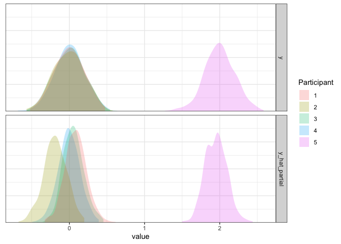
As we can see, the fit is extremely good given our limited data. If you
look closely, there’s one slight discrepency, however. Whereas most
participants’ estimates are on the nose, the outlier is pulled slightly
towards 0, the grand mean. Since the adjustments tend to be small this
might be hard to tell from the plot above, but it’s easier to see if we
directly compare the estimated means (using the nifty coef function)
with the raw means from the subsetted data:
1
2
3
d4 %>% group_by(participant) %>%
    summarize(y=mean(y)) %>%
    mutate(y_hat=coef(m4)$participant$`(Intercept)`)
1
2
3
4
5
6
7
8
## # A tibble: 5 × 3
##   participant        y    y_hat
##   <fct>          <dbl>    <dbl>
## 1 1            0.0880   0.0919
## 2 2           -0.191   -0.184
## 3 3            0.0518   0.0562
## 4 4           -0.00768 -0.00251
## 5 5            1.98     1.96
The reason this happens is because we assumed that participants will be somewhat similar, following a normal distribution. So, even though we don’t have a lot of data per participants, we can learn about each individual participant by looking at all of the other participants’ data! This is what makes multilevel models cool: it gives us the flexibility to model participant-level variation, while still affording us as much statistical power as we can get.
Conclusions
Whenever you have repeated-measures data, multilevel models are a great candidate for your analysis. They are the perfect medium between modeling each participant separately (for scientific interpretation) and modeling them as identical (for statistical power), and they can strike this balance automatically without you having to worry about it. Moreover, they’re flexible enough to capture repeated measures across multiple factors (e.g., participants and stimuli), as well as participant-level differences in the effect of a manipulation. As a bonus, below is a quick description of how you can extend the multilevel model in these two ways.
For more information, I recommend looking here:
- Intro to Mixed Effects Regression in R
- Intro to Bayesian Regression in R
- Just use multilevel models for your pre/post RCT data
- Plotting partial pooling in mixed-effects models
Bonus material
Intercepts and slopes
The above simulations only dealt with the simple case where you want to estimate the mean of some variable with participant-level differences. But what if we also have a (continuous or categorical) manipulation?
If the manipulation is between-participants (each participant only sees
one condition), then you can include that predictor just as usual. For
instance, you would end up with a lmer formula that looks something
like this: y ~ condition + (1 | participant).
If the manipulation is within-participants, then you will also likely
want to include a participant-level coefficient for condition,
resulting in a formula that looks like this:
y ~ condition + (condition | participant). The only exception is that
if you don’t have many trials per participant per condition, you may
want to treat condition as if it were a between-participant
manipulation. What does this syntax mean? Well, remember our assumption
that the participant means were normally distributed? Here we are also
assuming that the effect of condition for each participant is also
normally distributed. Specifically, we’re swapping out our univariate
normal distribution over intercepts for a bivariate normal distribution
over intercepts and slopes! Our equations now look like this:
Here \(\mathbf{\mu_p}\) is a vector containing the mean intercept and the mean effect of condition, averaging over all participants. Likewise, \(\Sigma_p\) is now a covariance matrix: it will be composed of the participant-level standard deviation around the intercept, the participant-level standard deviation around the effect of condition, and the participant-level correlation between the intercept and the effect of condition.
I won’t explain it in detail (maybe a future blog post?), but here is code to simulate & analyze data with a one-way repeated-measures design including participant-level intercepts and slopes:
1
2
3
4
5
6
7
8
9
10
11
12
13
14
15
16
17
18
19
20
21
22
23
24
25
26
27
28
29
30
31
32
33
library(mvtnorm)

N_participants <- 100  ## increase number of participants
N_trials <- 10

ALPHA <- 0            ## population-level intercept (mean for control)
BETA <- 1             ## population-level slope (mean effect of condition)

SIGMA_ALPHA <- .25    ## SD of participant-level intercepts
SIGMA_BETA <- .4      ## SD of participant-level slopes
RHO <- .7             ## correlation between participant-level intercepts & slopes

## Combine participant-level SDs & correlations into a covariance matrix
s <- diag(c(SIGMA_ALPHA, SIGMA_BETA))
SIGMA_P <- s %*% matrix(c(1, RHO, RHO, 1), nrow=2) %*% s

d5 <- expand_grid(participant=as.factor(1:N_participants),
                  condition=as.factor(c('control', 'treatment')),
                  trial=as.factor(1:N_trials)) %>%

    ## simulate a participant-level intercept and slope
    group_by(participant) %>%
    mutate(a=list(rmvnorm(1, mean=c(ALPHA, BETA), sigma=SIGMA_P)),
           alpha_p=map_dbl(a, ~ .[,1]),
           beta_p=map_dbl(a, ~ .[,2])) %>%

    ## simulate ratings based on participant-level effects
    ungroup() %>%
    mutate(y=rnorm(n(), mean=alpha_p + beta_p*(condition=='treatment'), sd=SIGMA))

## analyze data
m5 <- lmer(y ~ condition + (condition | participant), d5)
summary(m5)
1
2
3
4
5
6
7
8
9
10
11
12
13
14
15
16
17
18
19
20
21
22
23
24
25
## Linear mixed model fit by REML ['lmerMod']
## Formula: y ~ condition + (condition | participant)
##    Data: d5
##
## REML criterion at convergence: -96.1
##
## Scaled residuals:
##     Min      1Q  Median      3Q     Max
## -2.9935 -0.6684 -0.0136  0.6326  3.2471
##
## Random effects:
##  Groups      Name               Variance Std.Dev. Corr
##  participant (Intercept)        0.06394  0.2529
##              conditiontreatment 0.17160  0.4142   0.74
##  Residual                       0.04116  0.2029
## Number of obs: 2000, groups:  participant, 100
##
## Fixed effects:
##                    Estimate Std. Error t value
## (Intercept)        -0.02033    0.02609  -0.779
## conditiontreatment  0.92014    0.04241  21.698
##
## Correlation of Fixed Effects:
##             (Intr)
## cndtntrtmnt 0.664
In this case, the intercept, slope, residual standard deviation, and participant-level covariance matrix are estimated well! Note, though, that you need more participants to estimate the participant-level correlations than to estimate the intercepts/slopes themselves.
Multiple repeated factors
Another common extension of multilevel models is to include individual effects for more than one grouping variable. For instance, we might be interested not only in differences in means between participants, but also between the individual stimuli shown to participants. Thankfully, accomodating stimulus effects is really easy- we just have to add another normally-distributed effect per stimulus!
\[\begin{align*} y_n &\sim \mathcal{N}(\alpha_{p[n]} + \gamma_{s[n]}, \sigma) \\ \alpha_{p} &\sim \mathcal{N}(\mu_p, \sigma_p) \\ \gamma_{s} &\sim \mathcal{N}(\mu_s, \sigma_s) \end{align*}\]Estimating this model is also straightforward: we again just need to add the stimulus-level intercept term.
1
2
3
4
5
6
7
8
9
10
11
12
13
14
15
16
17
18
19
20
21
22
23
24
N_stimuli <- 50      ## number of unique stimuli
N_trials <- 5        ## number of trials per participant/simulus

SIGMA_ALPHA <- .25   ## participant-level SD
SIGMA_GAMMA <- .9    ## stimulus-level SD

d6 <- expand_grid(participant=as.factor(1:N_participants),
            stimulus=as.factor(1:N_stimuli),
            trial=as.factor(1:N_trials)) %>%

    ## simulate a partipant-level mean
    group_by(participant) %>%
    mutate(mu_p=rnorm(1, 0, SIGMA_ALPHA)) %>%

    ## simulate a stimulus-level mean
    group_by(stimulus) %>%
    mutate(mu_s=rnorm(1, 0, SIGMA_GAMMA)) %>%

    ## simulate responses from participant/stimulus-level means
    ungroup() %>%
    mutate(y=rnorm(n(), ALPHA + mu_p + mu_s, sd=SIGMA))

m6 <- lmer(y ~ 1 + (1 | participant) + (1 | stimulus), d6)
summary(m6)
1
2
3
4
5
6
7
8
9
10
11
12
13
14
15
16
17
18
19
20
## Linear mixed model fit by REML ['lmerMod']
## Formula: y ~ 1 + (1 | participant) + (1 | stimulus)
##    Data: d6
##
## REML criterion at convergence: -8446.4
##
## Scaled residuals:
##     Min      1Q  Median      3Q     Max
## -5.0902 -0.6724 -0.0083  0.6676  3.6152
##
## Random effects:
##  Groups      Name        Variance Std.Dev.
##  participant (Intercept) 0.05539  0.2354
##  stimulus    (Intercept) 0.78635  0.8868
##  Residual                0.04006  0.2002
## Number of obs: 25000, groups:  participant, 100; stimulus, 50
##
## Fixed effects:
##             Estimate Std. Error t value
## (Intercept)  -0.1621     0.1276   -1.27