Hidden Markov Models
Hidden Markov Models (HMMs) are statistical tools that are well-known for their ability to capture heterogeneous patterns in data over time, to reproduce text and gene sequences, and to identify interpretable factors underlying variation. However, since many introductory statistics courses never cover HMMs (and those that do usually fail to apply them to practical datasets of interest), many people have the impression that they are too complicated or burdensome to be applied in standard analyses in fields like psychology and neuroscience. In this tutorial, we’re going to break down what HMMs are, why they are popular in computational fields, and how you can apply them in your own research.
Note: I’ll be using the languages R and Stan to demonstrate HMMs, but there are many great packages for fitting them in other languages with other estimation techniques. To make this tutorial, I used the Stan User’s Guide and this fantastic paper by Luis Damiano as references.
- Standard Models
- Mixture Models
- Hidden Markov Models
- Simulating from HMMs
- Supervised learning
- Unsupervised learning
- Conclusions
Standard Models
To understand what HMMs are and how they differ from more well-known types of models, let’s start with a dirt-simple model, and see if we can build up step-by-step until we get a HMM. Here we are going to focus on modeling reaction times from a single participant in a decision-making type of experment inspired by a cool model by Martin Modrak. The data we’ll be using were simulated, but the same sorts of analyses will apply to pretty much any cognitive task where reaction times are measured.
Let’s begin by loading our data in and taking a look at what they look like:
1
2
3
4
5
6
7
8
9
10
11
library(cmdstanr) # for stan
library(tidyverse) # for data wrangling
library(tidybayes) # for accessing model posteriors
library(patchwork) # for multi-plots
options(mc.cores=parallel::detectCores())
rts <- read_csv('2022-02-21-reaction-times.csv')
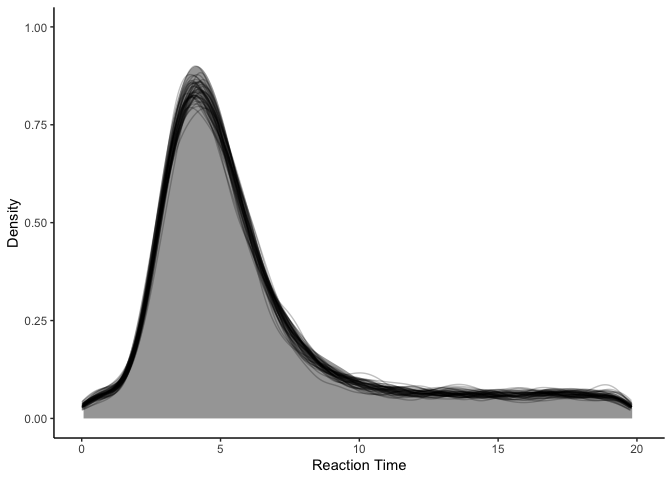
ggplot(rts, aes(x=rt)) +
stat_slab() + xlab('Reaction Time') + ylab('Density') +
theme_classic()
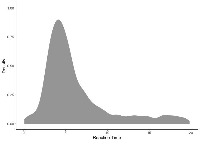
Looking at the data, it appears that our reaction times were generally around 4-5 seconds, but range anywhere from 0 to 20 seconds. Since these reaction times are clearly skewed, we’re going to model them using a lognormal distribution rather than a normal distribution:
\[log(rt_i) \sim \mathcal{N}(\mu, \sigma)\]or simply
\[rt_i \sim lognormal(\mu, \sigma)\]This formula says that the log-ed reaction times should be normally distributed around μ with standard deviation σ . More generally, standard models of data will look something like this:
\[y_i \sim \mathcal{D}(\theta)\]where 𝒟 is the data-generating distribution and θ are the parameters to distribution 𝒟 (like the mean and standard deviation of a normal distribution). To fit the model, we can write it into a simple stan program:
1
2
model.lognormal <- cmdstan_model('2022-02-21-lognormal.stan')
model.lognormal
1
2
3
4
5
6
7
8
9
10
11
12
13
14
15
16
17
18
19
20
21
22
23
data {
  int<lower=0> N;             // number of data points
  vector<lower=0>[N] y;       // data points
}

parameters {
  real mu;                    // lognormal location
  real<lower=0> sigma;        // lognormal scale
}

model {
  mu ~ std_normal();
  sigma ~ std_normal();
  y ~ lognormal(mu, sigma);
}

generated quantities {
  // simulated data points
  vector<lower=0>[N] y_rep;

  for (n in 1:N)
    y_rep[n] = lognormal_rng(mu, sigma);
}
If this doesn’t make any sense to you, I would recommend taking a look at my recent introduction to Stan, which explains the basics of the Stan probabilistic programming language. But generally this says the same thing as our formula above: we are estimating the parameters μ and σ of the lognormal distribution to best fit to our data. Let’s see how it works:
1
2
fit.lognormal <- model.lognormal$sample(data=list(N=nrow(rts), y=rts$rt))
fit.lognormal$summary(c('mu', 'sigma'))
1
2
3
4
5
6
7
8
9
10
11
12
13
14
15
16
17
18
19
20
21
22
23
24
25
26
27
28
29
30
31
32
33
34
35
36
37
38
39
40
41
42
43
44
45
46
47
48
49
50
51
52
53
54
55
56
57
58
59
60
61
62
63
64
65
66
67
68
69
70
71
72
73
74
75
76
77
78
79
80
81
82
83
84
85
86
87
88
89
90
91
92
93
94
95
96
97
98
99
100
101
102
103
## Running MCMC with 4 chains, at most 20 in parallel...
##
## Chain 1 Iteration:    1 / 2000 [  0%]  (Warmup)
## Chain 1 Iteration:  100 / 2000 [  5%]  (Warmup)
## Chain 1 Iteration:  200 / 2000 [ 10%]  (Warmup)
## Chain 1 Iteration:  300 / 2000 [ 15%]  (Warmup)
## Chain 1 Iteration:  400 / 2000 [ 20%]  (Warmup)
## Chain 1 Iteration:  500 / 2000 [ 25%]  (Warmup)
## Chain 1 Iteration:  600 / 2000 [ 30%]  (Warmup)
## Chain 1 Iteration:  700 / 2000 [ 35%]  (Warmup)
## Chain 1 Iteration:  800 / 2000 [ 40%]  (Warmup)
## Chain 1 Iteration:  900 / 2000 [ 45%]  (Warmup)
## Chain 1 Iteration: 1000 / 2000 [ 50%]  (Warmup)
## Chain 1 Iteration: 1001 / 2000 [ 50%]  (Sampling)
## Chain 2 Iteration:    1 / 2000 [  0%]  (Warmup)
## Chain 2 Iteration:  100 / 2000 [  5%]  (Warmup)
## Chain 2 Iteration:  200 / 2000 [ 10%]  (Warmup)
## Chain 2 Iteration:  300 / 2000 [ 15%]  (Warmup)
## Chain 2 Iteration:  400 / 2000 [ 20%]  (Warmup)
## Chain 2 Iteration:  500 / 2000 [ 25%]  (Warmup)
## Chain 2 Iteration:  600 / 2000 [ 30%]  (Warmup)
## Chain 2 Iteration:  700 / 2000 [ 35%]  (Warmup)
## Chain 2 Iteration:  800 / 2000 [ 40%]  (Warmup)
## Chain 2 Iteration:  900 / 2000 [ 45%]  (Warmup)
## Chain 2 Iteration: 1000 / 2000 [ 50%]  (Warmup)
## Chain 2 Iteration: 1001 / 2000 [ 50%]  (Sampling)
## Chain 3 Iteration:    1 / 2000 [  0%]  (Warmup)
## Chain 3 Iteration:  100 / 2000 [  5%]  (Warmup)
## Chain 3 Iteration:  200 / 2000 [ 10%]  (Warmup)
## Chain 3 Iteration:  300 / 2000 [ 15%]  (Warmup)
## Chain 3 Iteration:  400 / 2000 [ 20%]  (Warmup)
## Chain 3 Iteration:  500 / 2000 [ 25%]  (Warmup)
## Chain 3 Iteration:  600 / 2000 [ 30%]  (Warmup)
## Chain 3 Iteration:  700 / 2000 [ 35%]  (Warmup)
## Chain 3 Iteration:  800 / 2000 [ 40%]  (Warmup)
## Chain 3 Iteration:  900 / 2000 [ 45%]  (Warmup)
## Chain 3 Iteration: 1000 / 2000 [ 50%]  (Warmup)
## Chain 3 Iteration: 1001 / 2000 [ 50%]  (Sampling)
## Chain 3 Iteration: 1100 / 2000 [ 55%]  (Sampling)
## Chain 4 Iteration:    1 / 2000 [  0%]  (Warmup)
## Chain 4 Iteration:  100 / 2000 [  5%]  (Warmup)
## Chain 4 Iteration:  200 / 2000 [ 10%]  (Warmup)
## Chain 4 Iteration:  300 / 2000 [ 15%]  (Warmup)
## Chain 4 Iteration:  400 / 2000 [ 20%]  (Warmup)
## Chain 4 Iteration:  500 / 2000 [ 25%]  (Warmup)
## Chain 4 Iteration:  600 / 2000 [ 30%]  (Warmup)
## Chain 4 Iteration:  700 / 2000 [ 35%]  (Warmup)
## Chain 4 Iteration:  800 / 2000 [ 40%]  (Warmup)
## Chain 4 Iteration:  900 / 2000 [ 45%]  (Warmup)
## Chain 4 Iteration: 1000 / 2000 [ 50%]  (Warmup)
## Chain 4 Iteration: 1001 / 2000 [ 50%]  (Sampling)
## Chain 4 Iteration: 1100 / 2000 [ 55%]  (Sampling)
## Chain 1 Iteration: 1100 / 2000 [ 55%]  (Sampling)
## Chain 1 Iteration: 1200 / 2000 [ 60%]  (Sampling)
## Chain 1 Iteration: 1300 / 2000 [ 65%]  (Sampling)
## Chain 2 Iteration: 1100 / 2000 [ 55%]  (Sampling)
## Chain 2 Iteration: 1200 / 2000 [ 60%]  (Sampling)
## Chain 3 Iteration: 1200 / 2000 [ 60%]  (Sampling)
## Chain 4 Iteration: 1200 / 2000 [ 60%]  (Sampling)
## Chain 1 Iteration: 1400 / 2000 [ 70%]  (Sampling)
## Chain 2 Iteration: 1300 / 2000 [ 65%]  (Sampling)
## Chain 2 Iteration: 1400 / 2000 [ 70%]  (Sampling)
## Chain 3 Iteration: 1300 / 2000 [ 65%]  (Sampling)
## Chain 3 Iteration: 1400 / 2000 [ 70%]  (Sampling)
## Chain 4 Iteration: 1300 / 2000 [ 65%]  (Sampling)
## Chain 1 Iteration: 1500 / 2000 [ 75%]  (Sampling)
## Chain 2 Iteration: 1500 / 2000 [ 75%]  (Sampling)
## Chain 3 Iteration: 1500 / 2000 [ 75%]  (Sampling)
## Chain 4 Iteration: 1400 / 2000 [ 70%]  (Sampling)
## Chain 4 Iteration: 1500 / 2000 [ 75%]  (Sampling)
## Chain 1 Iteration: 1600 / 2000 [ 80%]  (Sampling)
## Chain 2 Iteration: 1600 / 2000 [ 80%]  (Sampling)
## Chain 3 Iteration: 1600 / 2000 [ 80%]  (Sampling)
## Chain 4 Iteration: 1600 / 2000 [ 80%]  (Sampling)
## Chain 1 Iteration: 1700 / 2000 [ 85%]  (Sampling)
## Chain 2 Iteration: 1700 / 2000 [ 85%]  (Sampling)
## Chain 3 Iteration: 1700 / 2000 [ 85%]  (Sampling)
## Chain 4 Iteration: 1700 / 2000 [ 85%]  (Sampling)
## Chain 1 Iteration: 1800 / 2000 [ 90%]  (Sampling)
## Chain 1 Iteration: 1900 / 2000 [ 95%]  (Sampling)
## Chain 2 Iteration: 1800 / 2000 [ 90%]  (Sampling)
## Chain 3 Iteration: 1800 / 2000 [ 90%]  (Sampling)
## Chain 4 Iteration: 1800 / 2000 [ 90%]  (Sampling)
## Chain 1 Iteration: 2000 / 2000 [100%]  (Sampling)
## Chain 2 Iteration: 1900 / 2000 [ 95%]  (Sampling)
## Chain 2 Iteration: 2000 / 2000 [100%]  (Sampling)
## Chain 3 Iteration: 1900 / 2000 [ 95%]  (Sampling)
## Chain 3 Iteration: 2000 / 2000 [100%]  (Sampling)
## Chain 4 Iteration: 1900 / 2000 [ 95%]  (Sampling)
## Chain 1 finished in 0.9 seconds.
## Chain 2 finished in 1.0 seconds.
## Chain 3 finished in 0.9 seconds.
## Chain 4 Iteration: 2000 / 2000 [100%]  (Sampling)
## Chain 4 finished in 1.0 seconds.
##
## All 4 chains finished successfully.
## Mean chain execution time: 1.0 seconds.
## Total execution time: 1.1 seconds.
## # A tibble: 2 × 10
##   variable  mean median      sd     mad    q5   q95  rhat ess_bulk ess_tail
##   <chr>    <dbl>  <dbl>   <dbl>   <dbl> <dbl> <dbl> <dbl>    <dbl>    <dbl>
## 1 mu       1.64   1.64  0.0125  0.0124  1.62  1.66   1.00    3981.    2548.
## 2 sigma    0.639  0.639 0.00897 0.00932 0.625 0.654  1.00    3259.    2386.
It looks like the model fit well enough, with μ = 1.6 and σ = 0.64 . Let’s plot model predictions against our data to get a sense of how well it fits:
1
2
3
4
5
6
7
8
fit.lognormal %>%
    spread_draws(y_rep[.row], ndraws=50) %>%
    ggplot(aes(x=y_rep)) +
    stat_slab(aes(x=rt), data=rts) +
    stat_slab(aes(group=.draw), color='black', fill=NA, alpha=0.25, slab_size=.5) +
    coord_cartesian(xlim=c(0, 20)) +
    xlab('Reaction Time') + ylab('Density') +
    theme_classic()
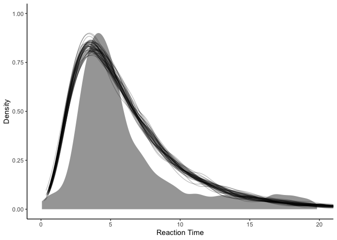
Sadly, while our model (black lines) captures the mode pretty well, it seems to overestimate the variance, such that it predicts that really short and really long reaction times are more likely than they should be.
Mixture Models
To improve our model, we it is worth looking closely at our data in the plot above. Something stands out to me: whereas the most of the reaction times look like they would be well-captured by a lognormal model, they seem to be “contaminated” by a whole bunch of really long and really short reaction times. There are two main approaches to handle this kind of data. The most common approach would be to simply discard any reaction times that are deemed “too short” or “too long.” While this is probably the most common way of dealing with it, it comes with some problems. First, we have to specify arbitrary thresholds a priori to throw away data, and our results could very well vary depending on the specific thresholds we choose. Second, it is reasonable to assume that we can actually learn something from the contaminated data. Both of these issues make the second approach, mixture models, much more favorable.
In a mixture model, we augment our model by assuming that our data does not just come from one distribution 𝒟(θ) , but we acknowledge that it could come from one of D distributions 𝒟d(θd) :
\[y_i \sim \mathcal{D}_{d[i]}(\theta_{d[i]})\]In our particular case, we can think of the reaction times arising from two possible distributions. When people were attentive to our task, their reaction times should be lognormally-distributed, as before. But when they weren’t paying attention, they were guessing, and we can assume that their reaction times here will be uniformly-distributed. In total, our model will look like this:
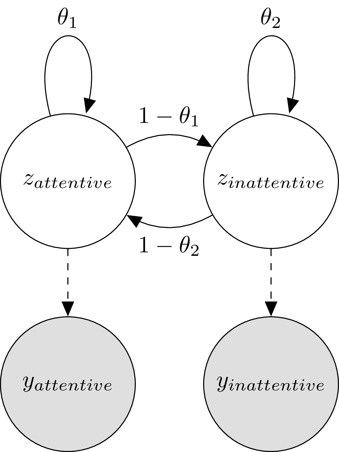
\[\begin{align*} z_i &\sim Bernoulli(\theta) \\ y_i &\sim \begin{cases} lognormal(\mu, \sigma) & z_i = 1 \\ uniform(0, y_max) & z_i = 2 \end{cases} \end{align*}\]The zi terms indicate for trial i , whether the participant was paying attention or not. We call this a latent or hidden variable, because we don’t have direct access to it: it is unobserved, and potentially unobservable (we can think of observing indicators of attentional state, but it is hard to say how we could measure it directly). Another way of representing the model is using a simple graph diagram:
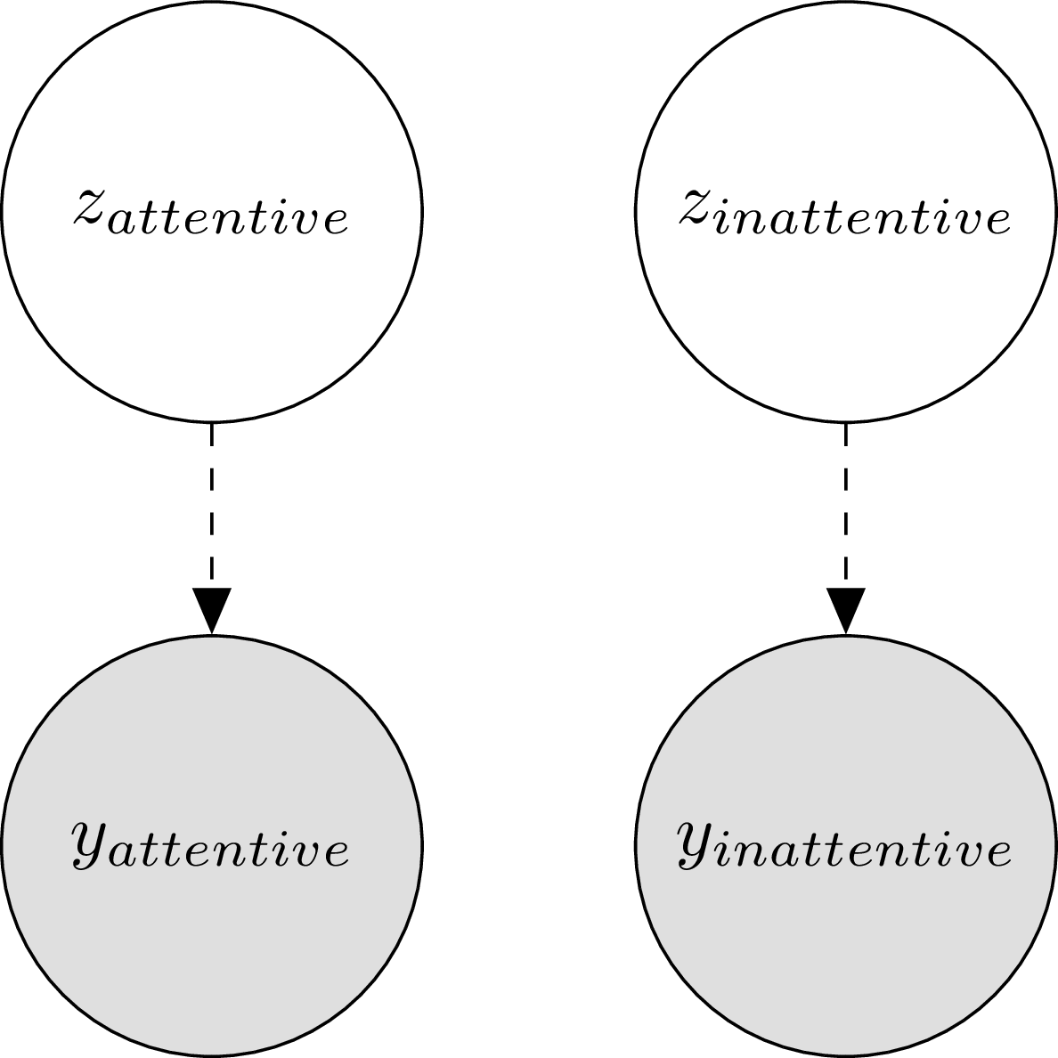
Under this representation, it’s clear that we’re assuming two possible latent states: an inattentive and an attentive state. Depending on which state we’re in, we’re going to get a different distribution of reaction times (though the graph doesn’t tell you exactly what those distributions are).
Thankfully, it is easy enough to program this mixture model in Stan:
1
2
model.mix <- cmdstan_model('2022-02-21-mixture.stan')
model.mix
1
2
3
4
5
6
7
8
9
10
11
12
13
14
15
16
17
18
19
20
21
22
23
24
25
26
27
28
29
30
31
32
33
34
35
36
37
38
39
40
data {
  int<lower=0> N;             // number of data points
  vector<lower=0>[N] y;       // data points
}

transformed data {
  real<lower=0> y_max = max(y);
}

parameters {
  real<lower=0, upper=1> theta;    // mixing proportion
  real mu;                         // lognormal location
  real<lower=0> sigma;             // lognormal scale
}

model {
  theta ~ uniform(0, 1);
  mu ~ std_normal();
  sigma ~ std_normal();

  for (n in 1:N) {
    target += log_mix(theta,
              lognormal_lpdf(y[n] | mu, sigma),
              uniform_lpdf(y[n] | 0, y_max));
  }
}

generated quantities {
  vector<lower=0, upper=1>[N] z_rep;   // simulated latent variables
  vector<lower=0>[N] y_rep;            // simulated data points

  for (n in 1:N) {
    z_rep[n] = bernoulli_rng(theta);

    if (z_rep[n] == 1)
      y_rep[n] = lognormal_rng(mu, sigma);
    else
      y_rep[n] = uniform_rng(0, y_max);
  }
}
Compared to before, we’ve added the data variable y_max which is
simply the upper bound for our reaction times, and theta which is the
probability of an observation coming from the lognormal distribution (as
opposed to the uniform distribution). The function log_mix lets us
define a mixture over the two distributions to calculate the log
likelihood. Finally, to simulate reaction times, we simulate whether the
observation came from the lognormal or not (z_rep), and then depending
on that value, we sample a reaction time. Let’s fit the model:
1
2
fit.mix <- model.mix$sample(data=list(N=nrow(rts), y=rts$rt))
fit.mix$summary(c('theta', 'mu', 'sigma'))
1
2
3
4
5
6
7
8
9
10
11
12
13
14
15
16
17
18
19
20
21
22
23
24
25
26
27
28
29
30
31
32
33
34
35
36
37
38
39
40
41
42
43
44
45
46
47
48
49
50
51
52
53
54
55
56
57
58
59
60
61
62
63
64
65
66
67
68
69
70
71
72
73
74
75
76
77
78
79
80
81
82
83
84
85
86
87
88
89
90
91
92
93
94
95
96
97
98
99
100
101
102
103
104
## Running MCMC with 4 chains, at most 20 in parallel...
##
## Chain 1 Iteration:    1 / 2000 [  0%]  (Warmup)
## Chain 2 Iteration:    1 / 2000 [  0%]  (Warmup)
## Chain 3 Iteration:    1 / 2000 [  0%]  (Warmup)
## Chain 4 Iteration:    1 / 2000 [  0%]  (Warmup)
## Chain 1 Iteration:  100 / 2000 [  5%]  (Warmup)
## Chain 2 Iteration:  100 / 2000 [  5%]  (Warmup)
## Chain 3 Iteration:  100 / 2000 [  5%]  (Warmup)
## Chain 4 Iteration:  100 / 2000 [  5%]  (Warmup)
## Chain 1 Iteration:  200 / 2000 [ 10%]  (Warmup)
## Chain 2 Iteration:  200 / 2000 [ 10%]  (Warmup)
## Chain 3 Iteration:  200 / 2000 [ 10%]  (Warmup)
## Chain 4 Iteration:  200 / 2000 [ 10%]  (Warmup)
## Chain 4 Iteration:  300 / 2000 [ 15%]  (Warmup)
## Chain 1 Iteration:  300 / 2000 [ 15%]  (Warmup)
## Chain 2 Iteration:  300 / 2000 [ 15%]  (Warmup)
## Chain 3 Iteration:  300 / 2000 [ 15%]  (Warmup)
## Chain 2 Iteration:  400 / 2000 [ 20%]  (Warmup)
## Chain 4 Iteration:  400 / 2000 [ 20%]  (Warmup)
## Chain 1 Iteration:  400 / 2000 [ 20%]  (Warmup)
## Chain 3 Iteration:  400 / 2000 [ 20%]  (Warmup)
## Chain 1 Iteration:  500 / 2000 [ 25%]  (Warmup)
## Chain 2 Iteration:  500 / 2000 [ 25%]  (Warmup)
## Chain 3 Iteration:  500 / 2000 [ 25%]  (Warmup)
## Chain 4 Iteration:  500 / 2000 [ 25%]  (Warmup)
## Chain 2 Iteration:  600 / 2000 [ 30%]  (Warmup)
## Chain 4 Iteration:  600 / 2000 [ 30%]  (Warmup)
## Chain 1 Iteration:  600 / 2000 [ 30%]  (Warmup)
## Chain 3 Iteration:  600 / 2000 [ 30%]  (Warmup)
## Chain 4 Iteration:  700 / 2000 [ 35%]  (Warmup)
## Chain 1 Iteration:  700 / 2000 [ 35%]  (Warmup)
## Chain 2 Iteration:  700 / 2000 [ 35%]  (Warmup)
## Chain 3 Iteration:  700 / 2000 [ 35%]  (Warmup)
## Chain 2 Iteration:  800 / 2000 [ 40%]  (Warmup)
## Chain 3 Iteration:  800 / 2000 [ 40%]  (Warmup)
## Chain 4 Iteration:  800 / 2000 [ 40%]  (Warmup)
## Chain 1 Iteration:  800 / 2000 [ 40%]  (Warmup)
## Chain 2 Iteration:  900 / 2000 [ 45%]  (Warmup)
## Chain 4 Iteration:  900 / 2000 [ 45%]  (Warmup)
## Chain 1 Iteration:  900 / 2000 [ 45%]  (Warmup)
## Chain 3 Iteration:  900 / 2000 [ 45%]  (Warmup)
## Chain 1 Iteration: 1000 / 2000 [ 50%]  (Warmup)
## Chain 1 Iteration: 1001 / 2000 [ 50%]  (Sampling)
## Chain 2 Iteration: 1000 / 2000 [ 50%]  (Warmup)
## Chain 2 Iteration: 1001 / 2000 [ 50%]  (Sampling)
## Chain 3 Iteration: 1000 / 2000 [ 50%]  (Warmup)
## Chain 3 Iteration: 1001 / 2000 [ 50%]  (Sampling)
## Chain 4 Iteration: 1000 / 2000 [ 50%]  (Warmup)
## Chain 4 Iteration: 1001 / 2000 [ 50%]  (Sampling)
## Chain 4 Iteration: 1100 / 2000 [ 55%]  (Sampling)
## Chain 1 Iteration: 1100 / 2000 [ 55%]  (Sampling)
## Chain 2 Iteration: 1100 / 2000 [ 55%]  (Sampling)
## Chain 3 Iteration: 1100 / 2000 [ 55%]  (Sampling)
## Chain 4 Iteration: 1200 / 2000 [ 60%]  (Sampling)
## Chain 1 Iteration: 1200 / 2000 [ 60%]  (Sampling)
## Chain 2 Iteration: 1200 / 2000 [ 60%]  (Sampling)
## Chain 3 Iteration: 1200 / 2000 [ 60%]  (Sampling)
## Chain 4 Iteration: 1300 / 2000 [ 65%]  (Sampling)
## Chain 1 Iteration: 1300 / 2000 [ 65%]  (Sampling)
## Chain 2 Iteration: 1300 / 2000 [ 65%]  (Sampling)
## Chain 3 Iteration: 1300 / 2000 [ 65%]  (Sampling)
## Chain 2 Iteration: 1400 / 2000 [ 70%]  (Sampling)
## Chain 4 Iteration: 1400 / 2000 [ 70%]  (Sampling)
## Chain 1 Iteration: 1400 / 2000 [ 70%]  (Sampling)
## Chain 3 Iteration: 1400 / 2000 [ 70%]  (Sampling)
## Chain 4 Iteration: 1500 / 2000 [ 75%]  (Sampling)
## Chain 2 Iteration: 1500 / 2000 [ 75%]  (Sampling)
## Chain 1 Iteration: 1500 / 2000 [ 75%]  (Sampling)
## Chain 3 Iteration: 1500 / 2000 [ 75%]  (Sampling)
## Chain 4 Iteration: 1600 / 2000 [ 80%]  (Sampling)
## Chain 2 Iteration: 1600 / 2000 [ 80%]  (Sampling)
## Chain 1 Iteration: 1600 / 2000 [ 80%]  (Sampling)
## Chain 3 Iteration: 1600 / 2000 [ 80%]  (Sampling)
## Chain 4 Iteration: 1700 / 2000 [ 85%]  (Sampling)
## Chain 2 Iteration: 1700 / 2000 [ 85%]  (Sampling)
## Chain 1 Iteration: 1700 / 2000 [ 85%]  (Sampling)
## Chain 3 Iteration: 1700 / 2000 [ 85%]  (Sampling)
## Chain 4 Iteration: 1800 / 2000 [ 90%]  (Sampling)
## Chain 2 Iteration: 1800 / 2000 [ 90%]  (Sampling)
## Chain 1 Iteration: 1800 / 2000 [ 90%]  (Sampling)
## Chain 3 Iteration: 1800 / 2000 [ 90%]  (Sampling)
## Chain 4 Iteration: 1900 / 2000 [ 95%]  (Sampling)
## Chain 2 Iteration: 1900 / 2000 [ 95%]  (Sampling)
## Chain 3 Iteration: 1900 / 2000 [ 95%]  (Sampling)
## Chain 1 Iteration: 1900 / 2000 [ 95%]  (Sampling)
## Chain 4 Iteration: 2000 / 2000 [100%]  (Sampling)
## Chain 4 finished in 4.7 seconds.
## Chain 2 Iteration: 2000 / 2000 [100%]  (Sampling)
## Chain 2 finished in 4.8 seconds.
## Chain 3 Iteration: 2000 / 2000 [100%]  (Sampling)
## Chain 3 finished in 4.9 seconds.
## Chain 1 Iteration: 2000 / 2000 [100%]  (Sampling)
## Chain 1 finished in 5.0 seconds.
##
## All 4 chains finished successfully.
## Mean chain execution time: 4.8 seconds.
## Total execution time: 5.2 seconds.
## # A tibble: 3 × 10
##   variable  mean median      sd     mad    q5   q95  rhat ess_bulk ess_tail
##   <chr>    <dbl>  <dbl>   <dbl>   <dbl> <dbl> <dbl> <dbl>    <dbl>    <dbl>
## 1 theta    0.709  0.709 0.0140  0.0141  0.686 0.732  1.00    2049.    2811.
## 2 mu       1.51   1.51  0.0103  0.00999 1.49  1.52   1.00    2760.    2970.
## 3 sigma    0.344  0.344 0.00901 0.00900 0.330 0.359  1.00    2254.    2605.
Everything is looking better! Our estimate for θ tells us that about 100% - 71% = 29% of our reaction times were contaminated, which is definitely more than just a little bit. A promising result is that σ seems to be smaller than before, which means that we might no longer be overestimating the variance. As before, we can plot simulated data from our model on top of the actual data to see how it looks:
1
2
3
4
5
6
7
8
fit.mix %>%
    spread_draws(y_rep[.row], ndraws=50) %>%
    ggplot(aes(x=y_rep)) +
    stat_slab(aes(x=rt), data=rts) +
    stat_slab(aes(group=.draw), color='black', fill=NA, alpha=0.25, slab_size=.5) +
    coord_cartesian(xlim=c(0, 20)) +
    xlab('Reaction Time') + ylab('Density') +
    theme_classic()

Wow! Our model fit has certainly improved, and in fact, it is difficult to find any obvious problems with it. So what could possibly be wrong with it? A closer inspection at our model might suggest some possibilities:
In hindsight, it seems a little weird that we’re estimating the latent state z to be independent on every trial. That is, our model simply says that ~70% of the time people were paying attention, and ~30% of the time they were guessing. But it would be odd if people suddenly bounced back and forth between an attentive and an inattentive state. In contrast, we should expect that the attentive trials should cluster in time, such that the participant went through extended periods of being attentive compared to not.
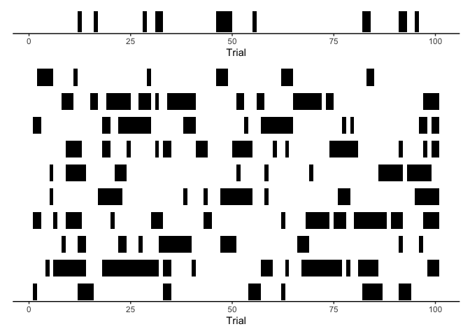
Since these data were simulated, we actually have access to whether the
participant was paying attention on a given trial (the column z in our
dataframe). To get an idea of whether our model is capturing the
attentiveness of our participant over time, we can compare the
participant’s actual timecourse of attention with our model predictions.
Here, let’s shade regions black during periods of inattention, leaving
periods of attention white:
1
2
3
4
5
6
7
8
9
10
11
12
13
14
15
16
17
18
19
20
21
22
p.data <- rts %>% filter(trial <= 100) %>%
    ggplot(aes(x=trial, y=1-z)) +
    geom_rect(aes(xmin=trial, xmax=trial+1, ymin=0, ymax=1-z), fill='black') +
    theme_classic()

p.model <- fit.mix %>%
    spread_draws(z_rep[trial], ndraws=10) %>%
    filter(trial <= 100) %>%
    ggplot(aes(x=trial, y=1-z_rep)) +
    geom_rect(aes(group=.draw, xmin=trial, xmax=trial+1, ymin=0, ymax=1-z_rep), fill='black') +
    facet_grid(.draw ~ .) +
    theme_classic()

(p.data / p.model) +
    plot_layout(heights=c(1, 10)) &
    xlab('Trial') &
    theme(axis.title.y=element_blank(),
          axis.ticks.y=element_blank(),
          axis.text.y=element_blank(),
          axis.line.y=element_blank(),
          strip.background = element_blank(),
          strip.text = element_blank())
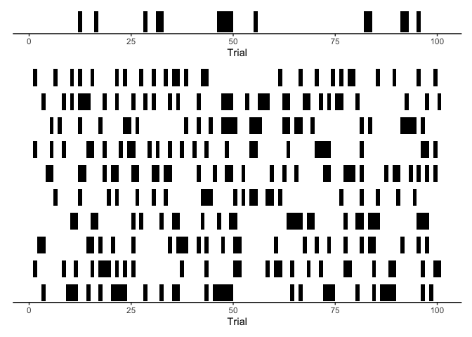
This is just a short period of time and a few of our posterior samples, but it should be clear that our model is missing something critical about human cognition: periods of inattention aren’t entirely random. To capture this behavior, we need HMMs.
Hidden Markov Models
HMMs expand on the basic idea of mixture models by allowing the latent states to vary over time. That is, instead of modeling each trial independently, HMMs model the entire sequence of trials all at once. To make things clear, let’s break down the name “Hidden Markov Model.”
First, what does it mean for an HMM to be “hidden?” Thankfully, this is actually the same as in our mixture model from before: “hidden” just refers to the fact that we’re assuming that our observations depend on some hidden, latent, or unobserved variable. In this case, our hidden variable is the participant’s attentive state.
Okay, then what does Markov refer to? A better question is “who does Markov refer to?” with the answer being mathematician Andrey Markov, who discovered what are now known as Markov chains. Markov chains are described by a graph with nodes referring to states and edges referring to transitions (with some probability). The key property of a Markov chain is that we start in one state, and our movement to the next state depends only on which state we are in. Importantly, where we move does not depend on which states we were in in the past, it only depends on the transition probabilities from the state we are in. In a HMM, the hidden or latent states form such a Markov chain. To make this concrete, we can expand our reaction time model to allow for transitions between attentive and inattentive states:

Hopefully you’ve noticed that the only difference to our model is that now the z states have edges between each other, as well as self-directed edges. You also probably noticed that the edges are labeled: instead of having a single mixture probability θ we now have two transition probabilities θ1 and θ2 . These determine the likelihood that the participant will remain attentive if they were attentive on the previous trial ( θ1 ) and the likelihood that they will remain inattentive if they were previously inattentive ( θ2 ). Since probabilities sum to one, the transition probabilities between attentive and inattentive states are just 1 − θ1 and 1 − θ2 .
In total, we now have four different transition probabilities, though each pair of probabilities is determined by just one unique parameter. A convenient way to represent these probabilities is using a matrix θ , where each element θi**j contains the transition probability from state i to state j :
\[\theta = \begin{bmatrix} \theta_1 & 1-\theta_1 \\ 1-\theta_2 & \theta_2 \end{bmatrix}\]Finally, the last thing we need is a probability distribution over the starting state, for which we’ll use a vector π :
\[\pi = \begin{bmatrix} \pi_1 & \pi_2 \end{bmatrix}\]In general π could take any form, but it’s often simplest to say that π is just the proportion spent in each state overall, called the stationary distribution of θ . I won’t go over the details here, but you can find the stationary distribution of θ by satisfying the linear equation π = π θ .
Given all of this information, another common way to think of HMMs is to “unroll” the graph above, using subscripts for time steps instead of state labels:
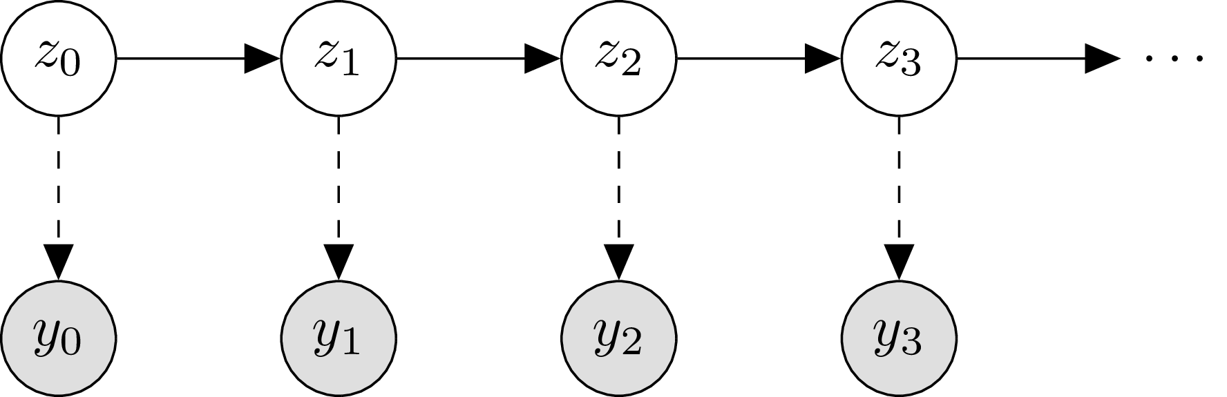
And that’s that! Now we have a formal model to capture temporal dynamics of reaction time distributions as a function of attentional state. Implementing this model, however, turns out to be more difficult than the models before. So, we’re going to go step by step, starting out with simulating sequences from the model using prior distributions.
Simulating from HMMs
Let’s start by programming in what we’ve just talked about to simulate from a prior distribution over reaction times from our HMM:
1
2
model.hmm.prior <- cmdstan_model('2022-02-21-hmm-sim.stan')
model.hmm.prior
1
2
3
4
5
6
7
8
9
10
11
12
13
14
15
16
17
18
19
20
21
22
23
24
25
26
27
28
29
30
31
32
33
34
35
36
37
38
39
40
41
42
43
44
45
46
47
48
49
50
51
52
53
54
55
56
57
58
59
60
61
62
63
64
65
66
67
68
69
70
71
72
73
74
75
functions {
  // get the log-likelihood of y given z, mu, sigma, and y_max
  real lognormal_mix_lpdf(real y, int z, real mu, real sigma, real y_max) {
    if (z == 1)
      return lognormal_lpdf(y | mu, sigma);
    else
      return uniform_lpdf(y | 0, y_max);
  }

  // simulate y given z, mu, sigma, and y_max
  real lognormal_mix_rng(int z, real mu, real sigma, real y_max) {
    if (z == 1)
      return lognormal_rng(mu, sigma);
    else
      return uniform_rng(0, y_max);
  }
}

data {
  int<lower=0> N;             // number of data points
  vector<lower=0>[N] y;       // data points
}

transformed data {
  int K = 2;                  // number of latent states (1=attentive, 2=guess)
  real y_max = max(y);        // maximum y value
}

parameters {
  array[K] simplex[K] theta;  // transition matrix

  real mu;                    // lognormal location
  real<lower=0> sigma;        // lognormal scale
}

transformed parameters {
  simplex[K] pi;              // starting probabilities

  {
    // copy theta to a matrix
    matrix[K, K] t;
    for(j in 1:K){
      for(i in 1:K){
    t[i,j] = theta[i,j];
      }
    }

    // solve for pi (assuming pi = pi * theta)
    pi = to_vector((to_row_vector(rep_vector(1.0, K))/
            (diag_matrix(rep_vector(1.0, K)) - t + rep_matrix(1, K, K))));
  }
}

model {
  for (k in 1:K)
    theta[k] ~ dirichlet([1, 1]');

  mu ~ std_normal();
  sigma ~ std_normal();
}

generated quantities {
  array[N] int<lower=1, upper=K> z_rep;   // simulated latent variables
  vector<lower=0>[N] y_rep;               // simulated data points

  // simulate starting state
  z_rep[1] = categorical_rng(pi);
  y_rep[1] = lognormal_mix_rng(z_rep[1], mu, sigma, y_max);

  // simulate forward
  for (n in 2:N) {
    z_rep[n] = categorical_rng(theta[z_rep[n-1]]);
    y_rep[n] = lognormal_mix_rng(z_rep[n], mu, sigma, y_max);
  }
}
The model here isn’t really all that different from the mixture model
earlier. As discussed above, theta is now a transition matrix instead
of a single probability, and pi is the expected proportion of time
spent in each state. We placed a
dirichlet prior
over each row of theta, which says that each row of theta should be
a simplex. To generate predictions from our model, we sample the first
latent state using a categorical distribution over pi, and then sample
subsequent states using a categorical distribution over
theta[z_rep[n-1]]. Note that I defined functions for our log
likelihood and random number generation to make things cleaner.
Since we aren’t actually modeling y yet (there is no likelihood for
y), this program just defines a prior distribution. Let’s sample from
this prior:
1
2
fit.hmm.prior <- model.hmm.prior$sample(data=list(N=nrow(rts), y=rts$rt))
fit.hmm.prior$summary(c('theta', 'pi', 'mu', 'sigma'))
1
2
3
4
5
6
7
8
9
10
11
12
13
14
15
16
17
18
19
20
21
22
23
24
25
26
27
28
29
30
31
32
33
34
35
36
37
38
39
40
41
42
43
44
45
46
47
48
49
50
51
52
53
54
55
56
57
58
59
60
61
62
63
64
65
66
67
68
69
70
71
72
73
74
75
76
77
78
79
80
81
82
83
84
85
86
87
88
89
90
91
92
93
94
95
96
97
98
99
100
101
102
103
104
105
106
107
108
109
## Running MCMC with 4 chains, at most 20 in parallel...
##
## Chain 1 Iteration:    1 / 2000 [  0%]  (Warmup)
## Chain 1 Iteration:  100 / 2000 [  5%]  (Warmup)
## Chain 1 Iteration:  200 / 2000 [ 10%]  (Warmup)
## Chain 1 Iteration:  300 / 2000 [ 15%]  (Warmup)
## Chain 1 Iteration:  400 / 2000 [ 20%]  (Warmup)
## Chain 1 Iteration:  500 / 2000 [ 25%]  (Warmup)
## Chain 1 Iteration:  600 / 2000 [ 30%]  (Warmup)
## Chain 1 Iteration:  700 / 2000 [ 35%]  (Warmup)
## Chain 1 Iteration:  800 / 2000 [ 40%]  (Warmup)
## Chain 1 Iteration:  900 / 2000 [ 45%]  (Warmup)
## Chain 1 Iteration: 1000 / 2000 [ 50%]  (Warmup)
## Chain 1 Iteration: 1001 / 2000 [ 50%]  (Sampling)
## Chain 2 Iteration:    1 / 2000 [  0%]  (Warmup)
## Chain 2 Iteration:  100 / 2000 [  5%]  (Warmup)
## Chain 2 Iteration:  200 / 2000 [ 10%]  (Warmup)
## Chain 2 Iteration:  300 / 2000 [ 15%]  (Warmup)
## Chain 2 Iteration:  400 / 2000 [ 20%]  (Warmup)
## Chain 2 Iteration:  500 / 2000 [ 25%]  (Warmup)
## Chain 2 Iteration:  600 / 2000 [ 30%]  (Warmup)
## Chain 2 Iteration:  700 / 2000 [ 35%]  (Warmup)
## Chain 2 Iteration:  800 / 2000 [ 40%]  (Warmup)
## Chain 2 Iteration:  900 / 2000 [ 45%]  (Warmup)
## Chain 2 Iteration: 1000 / 2000 [ 50%]  (Warmup)
## Chain 2 Iteration: 1001 / 2000 [ 50%]  (Sampling)
## Chain 3 Iteration:    1 / 2000 [  0%]  (Warmup)
## Chain 3 Iteration:  100 / 2000 [  5%]  (Warmup)
## Chain 3 Iteration:  200 / 2000 [ 10%]  (Warmup)
## Chain 3 Iteration:  300 / 2000 [ 15%]  (Warmup)
## Chain 3 Iteration:  400 / 2000 [ 20%]  (Warmup)
## Chain 3 Iteration:  500 / 2000 [ 25%]  (Warmup)
## Chain 3 Iteration:  600 / 2000 [ 30%]  (Warmup)
## Chain 3 Iteration:  700 / 2000 [ 35%]  (Warmup)
## Chain 3 Iteration:  800 / 2000 [ 40%]  (Warmup)
## Chain 3 Iteration:  900 / 2000 [ 45%]  (Warmup)
## Chain 3 Iteration: 1000 / 2000 [ 50%]  (Warmup)
## Chain 3 Iteration: 1001 / 2000 [ 50%]  (Sampling)
## Chain 4 Iteration:    1 / 2000 [  0%]  (Warmup)
## Chain 4 Iteration:  100 / 2000 [  5%]  (Warmup)
## Chain 4 Iteration:  200 / 2000 [ 10%]  (Warmup)
## Chain 4 Iteration:  300 / 2000 [ 15%]  (Warmup)
## Chain 4 Iteration:  400 / 2000 [ 20%]  (Warmup)
## Chain 4 Iteration:  500 / 2000 [ 25%]  (Warmup)
## Chain 4 Iteration:  600 / 2000 [ 30%]  (Warmup)
## Chain 4 Iteration:  700 / 2000 [ 35%]  (Warmup)
## Chain 4 Iteration:  800 / 2000 [ 40%]  (Warmup)
## Chain 4 Iteration:  900 / 2000 [ 45%]  (Warmup)
## Chain 4 Iteration: 1000 / 2000 [ 50%]  (Warmup)
## Chain 4 Iteration: 1001 / 2000 [ 50%]  (Sampling)
## Chain 1 Iteration: 1100 / 2000 [ 55%]  (Sampling)
## Chain 2 Iteration: 1100 / 2000 [ 55%]  (Sampling)
## Chain 3 Iteration: 1100 / 2000 [ 55%]  (Sampling)
## Chain 4 Iteration: 1100 / 2000 [ 55%]  (Sampling)
## Chain 1 Iteration: 1200 / 2000 [ 60%]  (Sampling)
## Chain 2 Iteration: 1200 / 2000 [ 60%]  (Sampling)
## Chain 4 Iteration: 1200 / 2000 [ 60%]  (Sampling)
## Chain 3 Iteration: 1200 / 2000 [ 60%]  (Sampling)
## Chain 1 Iteration: 1300 / 2000 [ 65%]  (Sampling)
## Chain 2 Iteration: 1300 / 2000 [ 65%]  (Sampling)
## Chain 3 Iteration: 1300 / 2000 [ 65%]  (Sampling)
## Chain 4 Iteration: 1300 / 2000 [ 65%]  (Sampling)
## Chain 1 Iteration: 1400 / 2000 [ 70%]  (Sampling)
## Chain 2 Iteration: 1400 / 2000 [ 70%]  (Sampling)
## Chain 4 Iteration: 1400 / 2000 [ 70%]  (Sampling)
## Chain 1 Iteration: 1500 / 2000 [ 75%]  (Sampling)
## Chain 3 Iteration: 1400 / 2000 [ 70%]  (Sampling)
## Chain 2 Iteration: 1500 / 2000 [ 75%]  (Sampling)
## Chain 3 Iteration: 1500 / 2000 [ 75%]  (Sampling)
## Chain 4 Iteration: 1500 / 2000 [ 75%]  (Sampling)
## Chain 1 Iteration: 1600 / 2000 [ 80%]  (Sampling)
## Chain 2 Iteration: 1600 / 2000 [ 80%]  (Sampling)
## Chain 4 Iteration: 1600 / 2000 [ 80%]  (Sampling)
## Chain 1 Iteration: 1700 / 2000 [ 85%]  (Sampling)
## Chain 3 Iteration: 1600 / 2000 [ 80%]  (Sampling)
## Chain 2 Iteration: 1700 / 2000 [ 85%]  (Sampling)
## Chain 3 Iteration: 1700 / 2000 [ 85%]  (Sampling)
## Chain 4 Iteration: 1700 / 2000 [ 85%]  (Sampling)
## Chain 1 Iteration: 1800 / 2000 [ 90%]  (Sampling)
## Chain 2 Iteration: 1800 / 2000 [ 90%]  (Sampling)
## Chain 4 Iteration: 1800 / 2000 [ 90%]  (Sampling)
## Chain 1 Iteration: 1900 / 2000 [ 95%]  (Sampling)
## Chain 3 Iteration: 1800 / 2000 [ 90%]  (Sampling)
## Chain 2 Iteration: 1900 / 2000 [ 95%]  (Sampling)
## Chain 3 Iteration: 1900 / 2000 [ 95%]  (Sampling)
## Chain 4 Iteration: 1900 / 2000 [ 95%]  (Sampling)
## Chain 1 Iteration: 2000 / 2000 [100%]  (Sampling)
## Chain 2 Iteration: 2000 / 2000 [100%]  (Sampling)
## Chain 4 Iteration: 2000 / 2000 [100%]  (Sampling)
## Chain 1 finished in 1.6 seconds.
## Chain 2 finished in 1.6 seconds.
## Chain 4 finished in 1.6 seconds.
## Chain 3 Iteration: 2000 / 2000 [100%]  (Sampling)
## Chain 3 finished in 1.7 seconds.
##
## All 4 chains finished successfully.
## Mean chain execution time: 1.6 seconds.
## Total execution time: 1.8 seconds.
## # A tibble: 8 × 10
##   variable     mean median    sd   mad      q5   q95  rhat ess_bulk ess_tail
##   <chr>       <dbl>  <dbl> <dbl> <dbl>   <dbl> <dbl> <dbl>    <dbl>    <dbl>
## 1 theta[1,1] 0.501  0.499  0.287 0.367  0.0547 0.949  1.00    3153.    2165.
## 2 theta[2,1] 0.494  0.500  0.292 0.379  0.0432 0.948  1.00    3563.    2173.
## 3 theta[1,2] 0.499  0.501  0.287 0.367  0.0512 0.945  1.00    3151.    2165.
## 4 theta[2,2] 0.506  0.500  0.292 0.379  0.0518 0.957  1.00    3563.    2173.
## 5 pi[1]      0.495  0.496  0.244 0.256  0.0762 0.911  1.00    2819.    2185.
## 6 pi[2]      0.505  0.504  0.244 0.256  0.0893 0.924  1.00    2819.    2185.
## 7 mu         0.0354 0.0403 0.993 1.00  -1.62   1.63   1.00    3750.    3012.
## 8 sigma      0.800  0.687  0.602 0.596  0.0596 1.95   1.00    2276.    1437.
As expected, all of the transition probabilities are close to .5. To get an idea of what the dynamics of the model look like, we can make a similar plot as before:
1
2
3
4
5
6
7
8
9
10
11
12
13
14
15
16
17
p.model <- fit.hmm.prior %>%
    spread_draws(z_rep[trial], ndraws=10) %>%
    filter(trial <= 100) %>%
    ggplot(aes(x=trial, y=1-z_rep)) +
    geom_rect(aes(group=.draw, xmin=trial, xmax=trial+1, ymin=0, ymax=1-z_rep), fill='black') +
    facet_grid(.draw ~ .) +
    theme_classic()

(p.data / p.model) +
    plot_layout(heights=c(1, 10)) &
    xlab('Trial') &
    theme(axis.title.y=element_blank(),
          axis.ticks.y=element_blank(),
          axis.text.y=element_blank(),
          axis.line.y=element_blank(),
          strip.background = element_blank(),
          strip.text = element_blank())
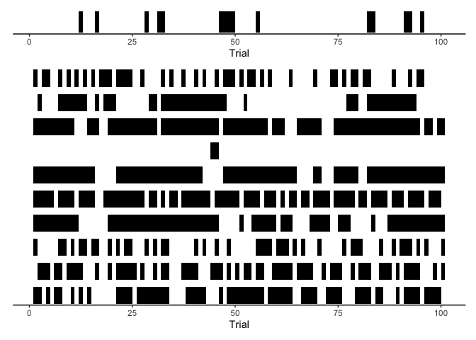
Clearly some of the prior samples look better than others, but overall we seem to have the potential to capture the behavior seen in our data. Next, we can try to fit the parameters of our model using data.
Supervised learning
In the best case scenario, we can imagine that we collected data for
both the observed variable
y
and the (not-so-latent-anymore) variable
z
. This is called the supervised learning problem for HMMs, because the
observed
z
’s can inform our choice of parameters. In the supervised learning case,
we can copy move our z_rep variable definition from the
generated quantities to the model block:
1
2
model.hmm.sup <- cmdstan_model('2022-02-21-hmm-sup.stan')
model.hmm.sup
1
2
3
4
5
6
7
8
9
10
11
12
13
14
15
16
17
18
19
20
21
22
23
24
25
26
27
28
29
30
31
32
33
34
35
36
37
38
39
40
41
42
43
44
45
46
47
48
49
50
51
52
53
54
55
56
57
58
59
60
61
62
63
64
65
66
67
68
69
70
71
72
73
74
75
76
77
78
79
80
81
82
83
84
85
86
functions {
  // get the log-likelihood of y given z, mu, sigma, and y_max
  real lognormal_mix_lpdf(real y, int z, real mu, real sigma, real y_max) {
    if (z == 1)
      return lognormal_lpdf(y | mu, sigma);
    else
      return uniform_lpdf(y | 0, y_max);
  }

  // simulate y given z, mu, sigma, and y_max
  real lognormal_mix_rng(int z, real mu, real sigma, real y_max) {
    if (z == 1)
      return lognormal_rng(mu, sigma);
    else
      return uniform_rng(0, y_max);
  }
}

data {
  int<lower=0> N;                         // number of data points
  array[N] int<lower=1, upper=2> z;       // hidden data points
  vector<lower=0>[N] y;                   // data points
}

transformed data {
  int K = 2;                  // number of latent states (1=attentive, 2=guess)
  real y_max = max(y);        // maximum y value
}

parameters {
  array[K] simplex[K] theta;  // transition matrix

  real mu;                    // lognormal location
  real<lower=0> sigma;        // lognormal scale
}

transformed parameters {
  simplex[K] pi;              // starting probabilities

  {
    // copy theta to a matrix
    matrix[K, K] t;
    for(j in 1:K){
      for(i in 1:K){
    t[i,j] = theta[i,j];
      }
    }

    // solve for pi (assuming pi = pi * theta)
    pi = to_vector((to_row_vector(rep_vector(1.0, K))/
            (diag_matrix(rep_vector(1.0, K)) - t + rep_matrix(1, K, K))));
  }
}

model {
  for (k in 1:K)
    theta[k] ~ dirichlet([1, 1]');

  mu ~ std_normal();
  sigma ~ std_normal();

  // likelihood for starting time
  z[1] ~ categorical(pi);
  y[1] ~ lognormal_mix(z[1], mu, sigma, y_max);

  // likelihood for subsequent times
  for (n in 2:N) {
    z[n] ~ categorical(theta[z[n-1]]);
    y[n] ~ lognormal_mix(z[n], mu, sigma, y_max);
  }
}

generated quantities {
  array[N] int<lower=1, upper=K> z_rep;   // simulated latent variables
  vector<lower=0>[N] y_rep;               // simulated data points

  // simulate starting state
  z_rep[1] = categorical_rng(pi);
  y_rep[1] = lognormal_mix_rng(z[1], mu, sigma, y_max);

  // simulate forward
  for (n in 2:N) {
    z_rep[n] = categorical_rng(theta[z_rep[n-1]]);
    y_rep[n] = lognormal_mix_rng(z[n], mu, sigma, y_max);
  }
}
Notice that we no longer need to use log_mix as we did for our mixture
model, because in the supervised case we know exactly which distribution
y[n] should be coming from. I also simulated our y_rep using the
actual zs instead of the simulated z_reps for the same reason. Let’s
fit the model:
1
2
fit.hmm.sup <- model.hmm.sup$sample(data=list(N=nrow(rts), y=rts$rt, z=rts$z))
fit.hmm.sup$summary(c('theta', 'pi', 'mu', 'sigma'))
1
2
3
4
5
6
7
8
9
10
11
12
13
14
15
16
17
18
19
20
21
22
23
24
25
26
27
28
29
30
31
32
33
34
35
36
37
38
39
40
41
42
43
44
45
46
47
48
49
50
51
52
53
54
55
56
57
58
59
60
61
62
63
64
65
66
67
68
69
70
71
72
73
74
75
76
77
78
79
80
81
82
83
84
85
86
87
88
89
90
91
92
93
94
95
96
97
98
99
100
101
102
103
104
105
106
107
108
109
## Running MCMC with 4 chains, at most 20 in parallel...
##
## Chain 1 Iteration:    1 / 2000 [  0%]  (Warmup)
## Chain 2 Iteration:    1 / 2000 [  0%]  (Warmup)
## Chain 3 Iteration:    1 / 2000 [  0%]  (Warmup)
## Chain 4 Iteration:    1 / 2000 [  0%]  (Warmup)
## Chain 1 Iteration:  100 / 2000 [  5%]  (Warmup)
## Chain 2 Iteration:  100 / 2000 [  5%]  (Warmup)
## Chain 3 Iteration:  100 / 2000 [  5%]  (Warmup)
## Chain 4 Iteration:  100 / 2000 [  5%]  (Warmup)
## Chain 1 Iteration:  200 / 2000 [ 10%]  (Warmup)
## Chain 3 Iteration:  200 / 2000 [ 10%]  (Warmup)
## Chain 2 Iteration:  200 / 2000 [ 10%]  (Warmup)
## Chain 1 Iteration:  300 / 2000 [ 15%]  (Warmup)
## Chain 2 Iteration:  300 / 2000 [ 15%]  (Warmup)
## Chain 3 Iteration:  300 / 2000 [ 15%]  (Warmup)
## Chain 4 Iteration:  200 / 2000 [ 10%]  (Warmup)
## Chain 1 Iteration:  400 / 2000 [ 20%]  (Warmup)
## Chain 2 Iteration:  400 / 2000 [ 20%]  (Warmup)
## Chain 3 Iteration:  400 / 2000 [ 20%]  (Warmup)
## Chain 4 Iteration:  300 / 2000 [ 15%]  (Warmup)
## Chain 1 Iteration:  500 / 2000 [ 25%]  (Warmup)
## Chain 2 Iteration:  500 / 2000 [ 25%]  (Warmup)
## Chain 3 Iteration:  500 / 2000 [ 25%]  (Warmup)
## Chain 4 Iteration:  400 / 2000 [ 20%]  (Warmup)
## Chain 1 Iteration:  600 / 2000 [ 30%]  (Warmup)
## Chain 2 Iteration:  600 / 2000 [ 30%]  (Warmup)
## Chain 3 Iteration:  600 / 2000 [ 30%]  (Warmup)
## Chain 1 Iteration:  700 / 2000 [ 35%]  (Warmup)
## Chain 4 Iteration:  500 / 2000 [ 25%]  (Warmup)
## Chain 2 Iteration:  700 / 2000 [ 35%]  (Warmup)
## Chain 3 Iteration:  700 / 2000 [ 35%]  (Warmup)
## Chain 4 Iteration:  600 / 2000 [ 30%]  (Warmup)
## Chain 1 Iteration:  800 / 2000 [ 40%]  (Warmup)
## Chain 2 Iteration:  800 / 2000 [ 40%]  (Warmup)
## Chain 3 Iteration:  800 / 2000 [ 40%]  (Warmup)
## Chain 4 Iteration:  700 / 2000 [ 35%]  (Warmup)
## Chain 1 Iteration:  900 / 2000 [ 45%]  (Warmup)
## Chain 2 Iteration:  900 / 2000 [ 45%]  (Warmup)
## Chain 3 Iteration:  900 / 2000 [ 45%]  (Warmup)
## Chain 4 Iteration:  800 / 2000 [ 40%]  (Warmup)
## Chain 1 Iteration: 1000 / 2000 [ 50%]  (Warmup)
## Chain 1 Iteration: 1001 / 2000 [ 50%]  (Sampling)
## Chain 2 Iteration: 1000 / 2000 [ 50%]  (Warmup)
## Chain 2 Iteration: 1001 / 2000 [ 50%]  (Sampling)
## Chain 4 Iteration:  900 / 2000 [ 45%]  (Warmup)
## Chain 3 Iteration: 1000 / 2000 [ 50%]  (Warmup)
## Chain 3 Iteration: 1001 / 2000 [ 50%]  (Sampling)
## Chain 4 Iteration: 1000 / 2000 [ 50%]  (Warmup)
## Chain 4 Iteration: 1001 / 2000 [ 50%]  (Sampling)
## Chain 1 Iteration: 1100 / 2000 [ 55%]  (Sampling)
## Chain 2 Iteration: 1100 / 2000 [ 55%]  (Sampling)
## Chain 3 Iteration: 1100 / 2000 [ 55%]  (Sampling)
## Chain 4 Iteration: 1100 / 2000 [ 55%]  (Sampling)
## Chain 1 Iteration: 1200 / 2000 [ 60%]  (Sampling)
## Chain 2 Iteration: 1200 / 2000 [ 60%]  (Sampling)
## Chain 3 Iteration: 1200 / 2000 [ 60%]  (Sampling)
## Chain 4 Iteration: 1200 / 2000 [ 60%]  (Sampling)
## Chain 1 Iteration: 1300 / 2000 [ 65%]  (Sampling)
## Chain 2 Iteration: 1300 / 2000 [ 65%]  (Sampling)
## Chain 3 Iteration: 1300 / 2000 [ 65%]  (Sampling)
## Chain 4 Iteration: 1300 / 2000 [ 65%]  (Sampling)
## Chain 2 Iteration: 1400 / 2000 [ 70%]  (Sampling)
## Chain 1 Iteration: 1400 / 2000 [ 70%]  (Sampling)
## Chain 3 Iteration: 1400 / 2000 [ 70%]  (Sampling)
## Chain 4 Iteration: 1400 / 2000 [ 70%]  (Sampling)
## Chain 2 Iteration: 1500 / 2000 [ 75%]  (Sampling)
## Chain 1 Iteration: 1500 / 2000 [ 75%]  (Sampling)
## Chain 3 Iteration: 1500 / 2000 [ 75%]  (Sampling)
## Chain 4 Iteration: 1500 / 2000 [ 75%]  (Sampling)
## Chain 1 Iteration: 1600 / 2000 [ 80%]  (Sampling)
## Chain 2 Iteration: 1600 / 2000 [ 80%]  (Sampling)
## Chain 3 Iteration: 1600 / 2000 [ 80%]  (Sampling)
## Chain 4 Iteration: 1600 / 2000 [ 80%]  (Sampling)
## Chain 1 Iteration: 1700 / 2000 [ 85%]  (Sampling)
## Chain 2 Iteration: 1700 / 2000 [ 85%]  (Sampling)
## Chain 3 Iteration: 1700 / 2000 [ 85%]  (Sampling)
## Chain 4 Iteration: 1700 / 2000 [ 85%]  (Sampling)
## Chain 1 Iteration: 1800 / 2000 [ 90%]  (Sampling)
## Chain 2 Iteration: 1800 / 2000 [ 90%]  (Sampling)
## Chain 3 Iteration: 1800 / 2000 [ 90%]  (Sampling)
## Chain 4 Iteration: 1800 / 2000 [ 90%]  (Sampling)
## Chain 2 Iteration: 1900 / 2000 [ 95%]  (Sampling)
## Chain 1 Iteration: 1900 / 2000 [ 95%]  (Sampling)
## Chain 3 Iteration: 1900 / 2000 [ 95%]  (Sampling)
## Chain 4 Iteration: 1900 / 2000 [ 95%]  (Sampling)
## Chain 2 Iteration: 2000 / 2000 [100%]  (Sampling)
## Chain 2 finished in 4.8 seconds.
## Chain 1 Iteration: 2000 / 2000 [100%]  (Sampling)
## Chain 1 finished in 4.8 seconds.
## Chain 3 Iteration: 2000 / 2000 [100%]  (Sampling)
## Chain 4 Iteration: 2000 / 2000 [100%]  (Sampling)
## Chain 3 finished in 4.9 seconds.
## Chain 4 finished in 4.9 seconds.
##
## All 4 chains finished successfully.
## Mean chain execution time: 4.9 seconds.
## Total execution time: 5.1 seconds.
## # A tibble: 8 × 10
##   variable    mean median      sd     mad     q5   q95  rhat ess_bulk ess_tail
##   <chr>      <dbl>  <dbl>   <dbl>   <dbl>  <dbl> <dbl> <dbl>    <dbl>    <dbl>
## 1 theta[1,1] 0.895  0.895 0.00741 0.00744 0.882  0.906  1.00    4668.    3425.
## 2 theta[2,1] 0.259  0.259 0.0165  0.0165  0.232  0.287  1.00    4140.    3101.
## 3 theta[1,2] 0.105  0.105 0.00741 0.00744 0.0939 0.118  1.00    4668.    3425.
## 4 theta[2,2] 0.741  0.741 0.0165  0.0165  0.713  0.768  1.00    4140.    3101.
## 5 pi[1]      0.710  0.710 0.0194  0.0198  0.678  0.741  1.00    4220.    3390.
## 6 pi[2]      0.290  0.290 0.0194  0.0198  0.259  0.322  1.00    4220.    3390.
## 7 mu         1.51   1.51  0.00827 0.00835 1.50   1.53   1.00    5384.    2775.
## 8 sigma      0.337  0.337 0.00571 0.00568 0.328  0.347  1.00    4877.    2903.
Comparing this to our mixture model above, we should immediately see
similarities. First, our estimates of mu and sigma are essentially
the same as before! Second, our estimate of pi corresponds very well
with our mixing probability theta from the mixture model. These two
things alone mean that our marginal distribution should be just as
impressive as before. Let’s check:
1
2
3
4
5
6
7
8
fit.hmm.sup %>%
    spread_draws(y_rep[.row], ndraws=50) %>%
    ggplot(aes(x=y_rep)) +
    stat_slab(aes(x=rt), data=rts) +
    stat_slab(aes(group=.draw), color='black', fill=NA, alpha=0.25, slab_size=.5) +
    coord_cartesian(xlim=c(0, 20)) +
    xlab('Reaction Time') + ylab('Density') +
    theme_classic()
Indeed, it looks great! Next, we can inspect theta to see our
transition probabilities. Remember that the diagonal of theta tells us
the probability of staying in a particular state: since these
probabilities are both above 0.5, we can expect our model to produce
trajectories that look much more like our data:
1
2
3
4
5
6
7
8
9
10
11
12
13
14
15
16
17
p.model <- fit.hmm.sup %>%
    spread_draws(z_rep[trial], ndraws=10) %>%
    filter(trial <= 100) %>%
    ggplot(aes(x=trial, y=1-z_rep)) +
    geom_rect(aes(group=.draw, xmin=trial, xmax=trial+1, ymin=0, ymax=1-z_rep), fill='black') +
    facet_grid(.draw ~ .) +
    theme_classic()

(p.data / p.model) +
    plot_layout(heights=c(1, 10)) &
    xlab('Trial') &
    theme(axis.title.y=element_blank(),
          axis.ticks.y=element_blank(),
          axis.text.y=element_blank(),
          axis.line.y=element_blank(),
          strip.background = element_blank(),
          strip.text = element_blank())
Indeed, this looks a lot like our data! As a final step, we can look at our simulated reaction times over time:
1
2
3
4
5
6
7
fit.hmm.sup %>%
    spread_draws(y_rep[trial], ndraws=50) %>%
    filter(trial <= 100) %>%
    ggplot(aes(x=trial, y=y_rep)) +
    geom_line(aes(group=.draw), alpha=.25, size=.5, color='red') +
    geom_line(aes(y=rt), data=filter(rts, trial<=100), size=2) +
    theme_classic() + ylab('Reaction Time')
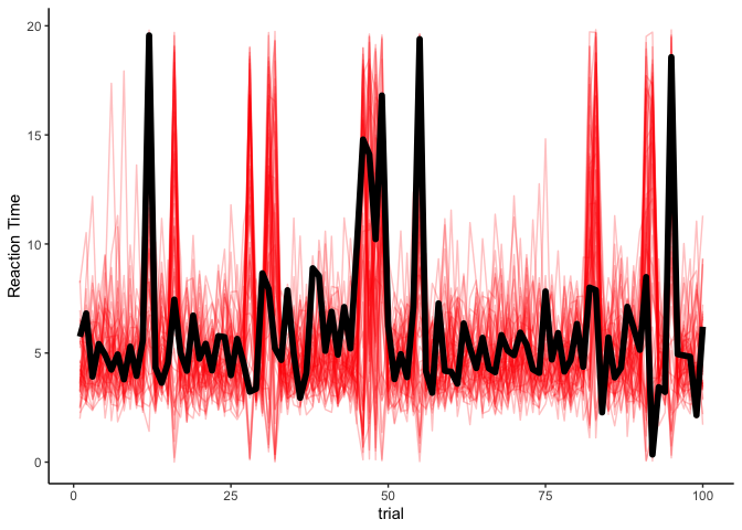
Although there is definitely some uncertainty, our model seems to be capturing the data very well. Thankfully, if we have observed the latent states, estimating an HMM is pretty straightforward.
Unsupervised learning
In the worst case (but probably most common) scenario, we don’t have any knowledge about the latent states z . In these cases, we must estimate the probability of latent states given our data. This is called a filtering problem in statistics, and it is customary to use what’s called the forward algorithm to solve it:
The forward algorithm
\[\begin{align*} p(z_t, y_{1:t}) &= \sum_{z_{t-1}} p(z_t, z_{t-1}, y_{1:t}) \\ &= \sum_{z_{t-1}} p(y_t | z_t, z_{t-1}, y_{1:(t-1)}) p(z_t | z_{t-1}, y_{1:(t-1)}) p(z_{t-1}, y_{1:(t-1)}) \\ &= \sum_{z_{t-1}} p(y_t | z_t) p(z_t | z_{t-1}) p(z_{t-1}, y_{1:(t-1)}) \\ &= p(y_t | z_t) \sum_{z_{t-1}} p(z_t | z_{t-1}) p(z_{t-1}, y_{1:(t-1)}) \end{align*}\]As you can see, we can express the joint probability of zt and y1 : t as a function of (i) the emission probability p(yt|zt) , (ii) the transition probability p(zt|zt − 1) , and (iii) the joint probability of zt − 1 and y1 : (t−1) , we can estimate these probabilities recursively by moving forward in time (hence, the forward algorithm). Given the joint probability of zt and y1 : t , it is simple to marginalize over the possible zt ’s to get the likelihood of the data.
We can code this directly into the model block of our Stan program as
follows (code provided in the Stan user
guide):
1
2
model.hmm <- cmdstan_model('2022-02-21-hmm.stan')
model.hmm
1
2
3
4
5
6
7
8
9
10
11
12
13
14
15
16
17
18
19
20
21
22
23
24
25
26
27
28
29
30
31
32
33
34
35
36
37
38
39
40
41
42
43
44
45
46
47
48
49
50
51
52
53
54
55
56
57
58
59
60
61
62
63
64
65
66
67
68
69
70
71
72
73
74
75
76
77
78
79
80
81
82
83
84
85
86
87
88
89
90
91
92
93
94
95
96
97
98
99
100
101
102
103
104
105
106
functions {
  // get the log-likelihood of y given z, mu, sigma, and y_max
  real lognormal_mix_lpdf(real y, int z, real mu, real sigma, real y_max) {
    if (z == 1)
      return lognormal_lpdf(y | mu, sigma);
    else
      return uniform_lpdf(y | 0, y_max);
  }

  // simulate y given z, mu, sigma, and y_max
  real lognormal_mix_rng(int z, real mu, real sigma, real y_max) {
    if (z == 1)
      return lognormal_rng(mu, sigma);
    else
      return uniform_rng(0, y_max);
  }

  // forward algorithm for calculating log-likelihood of y
  array[,] real forward(vector y, array[] vector theta, vector pi, real mu, real sigma, real y_max) {
    int N = size(y);
    int K = size(pi);

    array[K] real acc;       // temporary variable
    array[N, K] real alpha;  // log p(y[1:n], z[n]==k)

    // first observation
    for (k in 1:K)
      alpha[1, k] = log(pi[k]) + lognormal_mix_lpdf(y[1] | k, mu, sigma, y_max);

    for (n in 2:N) {
      for (k in 1:K) {
    for (j in 1:K) {
      // calculate log p(y[1:n], z[n]==k, z[n-1]==j)
      acc[j] = alpha[n-1, j] + log(theta[j, k]) +
        lognormal_mix_lpdf(y[n] | k, mu, sigma, y_max);
    }

    alpha[n, k] = log_sum_exp(acc);  // marginalize over all previous states j
      }
    }

    return alpha;
  }
}

data {
  int<lower=0> N;                         // number of data points
  vector<lower=0>[N] y;                   // data points
}

transformed data {
  int K = 2;                  // number of latent states (1=attentive, 2=guess)
  real y_max = max(y);        // maximum y value
}

parameters {
  array[K] simplex[K] theta;  // transition matrix

  real mu;                    // lognormal location
  real<lower=0> sigma;        // lognormal scale
}

transformed parameters {
  simplex[K] pi;              // starting probabilities

  {
    // copy theta to a matrix
    matrix[K, K] t;
    for(j in 1:K){
      for(i in 1:K){
    t[i,j] = theta[i,j];
      }
    }

    // solve for pi (assuming pi = pi * theta)
    pi = to_vector((to_row_vector(rep_vector(1.0, K))/
            (diag_matrix(rep_vector(1.0, K)) - t + rep_matrix(1, K, K))));
  }

  array[N, K] real alpha = forward(y, theta, pi, mu, sigma, y_max);
}

model {
  for (k in 1:K)
    theta[k] ~ dirichlet([1, 1]');

  mu ~ std_normal();
  sigma ~ std_normal();

  target += log_sum_exp(alpha[N]);     // marginalize over all ending states
}

generated quantities {
  array[N] int<lower=1, upper=K> z_rep;   // simulated latent variables
  vector<lower=0>[N] y_rep;               // simulated data points

  // simulate starting state
  z_rep[1] = categorical_rng(pi);
  y_rep[1] = lognormal_mix_rng(z_rep[1], mu, sigma, y_max);

  // simulate forward
  for (n in 2:N) {
    z_rep[n] = categorical_rng(theta[z_rep[n-1]]);
    y_rep[n] = lognormal_mix_rng(z_rep[n], mu, sigma, y_max);
  }
}
The only difference is that instead of evaluating the likelihood of y
as a function of some observed zs, we’re calculating the likelihood
recursively using the forward algorithm. I won’t go over the details of
how exactly it works (it is literally using the formula above), but now
we can fit the model:
1
2
fit.hmm <- model.hmm$sample(data=list(N=nrow(rts), y=rts$rt))
fit.hmm$summary(c('theta', 'pi', 'mu', 'sigma'))
1
2
3
4
5
6
7
8
9
10
11
12
13
14
15
16
17
18
19
20
21
22
23
24
25
26
27
28
29
30
31
32
33
34
35
36
37
38
39
40
41
42
43
44
45
46
47
48
49
50
51
52
53
54
55
56
57
58
59
60
61
62
63
64
65
66
67
68
69
70
71
72
73
74
75
76
77
78
79
80
81
82
83
84
85
86
87
88
89
90
91
92
93
94
95
96
97
98
99
100
101
102
103
104
105
106
107
108
109
## Running MCMC with 4 chains, at most 20 in parallel...
##
## Chain 1 Iteration:    1 / 2000 [  0%]  (Warmup)
## Chain 2 Iteration:    1 / 2000 [  0%]  (Warmup)
## Chain 3 Iteration:    1 / 2000 [  0%]  (Warmup)
## Chain 4 Iteration:    1 / 2000 [  0%]  (Warmup)
## Chain 1 Iteration:  100 / 2000 [  5%]  (Warmup)
## Chain 3 Iteration:  100 / 2000 [  5%]  (Warmup)
## Chain 2 Iteration:  100 / 2000 [  5%]  (Warmup)
## Chain 4 Iteration:  100 / 2000 [  5%]  (Warmup)
## Chain 3 Iteration:  200 / 2000 [ 10%]  (Warmup)
## Chain 1 Iteration:  200 / 2000 [ 10%]  (Warmup)
## Chain 4 Iteration:  200 / 2000 [ 10%]  (Warmup)
## Chain 3 Iteration:  300 / 2000 [ 15%]  (Warmup)
## Chain 2 Iteration:  200 / 2000 [ 10%]  (Warmup)
## Chain 1 Iteration:  300 / 2000 [ 15%]  (Warmup)
## Chain 3 Iteration:  400 / 2000 [ 20%]  (Warmup)
## Chain 4 Iteration:  300 / 2000 [ 15%]  (Warmup)
## Chain 1 Iteration:  400 / 2000 [ 20%]  (Warmup)
## Chain 2 Iteration:  300 / 2000 [ 15%]  (Warmup)
## Chain 4 Iteration:  400 / 2000 [ 20%]  (Warmup)
## Chain 3 Iteration:  500 / 2000 [ 25%]  (Warmup)
## Chain 2 Iteration:  400 / 2000 [ 20%]  (Warmup)
## Chain 1 Iteration:  500 / 2000 [ 25%]  (Warmup)
## Chain 4 Iteration:  500 / 2000 [ 25%]  (Warmup)
## Chain 3 Iteration:  600 / 2000 [ 30%]  (Warmup)
## Chain 1 Iteration:  600 / 2000 [ 30%]  (Warmup)
## Chain 2 Iteration:  500 / 2000 [ 25%]  (Warmup)
## Chain 4 Iteration:  600 / 2000 [ 30%]  (Warmup)
## Chain 3 Iteration:  700 / 2000 [ 35%]  (Warmup)
## Chain 1 Iteration:  700 / 2000 [ 35%]  (Warmup)
## Chain 2 Iteration:  600 / 2000 [ 30%]  (Warmup)
## Chain 4 Iteration:  700 / 2000 [ 35%]  (Warmup)
## Chain 1 Iteration:  800 / 2000 [ 40%]  (Warmup)
## Chain 3 Iteration:  800 / 2000 [ 40%]  (Warmup)
## Chain 2 Iteration:  700 / 2000 [ 35%]  (Warmup)
## Chain 4 Iteration:  800 / 2000 [ 40%]  (Warmup)
## Chain 3 Iteration:  900 / 2000 [ 45%]  (Warmup)
## Chain 1 Iteration:  900 / 2000 [ 45%]  (Warmup)
## Chain 2 Iteration:  800 / 2000 [ 40%]  (Warmup)
## Chain 4 Iteration:  900 / 2000 [ 45%]  (Warmup)
## Chain 3 Iteration: 1000 / 2000 [ 50%]  (Warmup)
## Chain 3 Iteration: 1001 / 2000 [ 50%]  (Sampling)
## Chain 1 Iteration: 1000 / 2000 [ 50%]  (Warmup)
## Chain 1 Iteration: 1001 / 2000 [ 50%]  (Sampling)
## Chain 2 Iteration:  900 / 2000 [ 45%]  (Warmup)
## Chain 4 Iteration: 1000 / 2000 [ 50%]  (Warmup)
## Chain 4 Iteration: 1001 / 2000 [ 50%]  (Sampling)
## Chain 2 Iteration: 1000 / 2000 [ 50%]  (Warmup)
## Chain 2 Iteration: 1001 / 2000 [ 50%]  (Sampling)
## Chain 1 Iteration: 1100 / 2000 [ 55%]  (Sampling)
## Chain 3 Iteration: 1100 / 2000 [ 55%]  (Sampling)
## Chain 4 Iteration: 1100 / 2000 [ 55%]  (Sampling)
## Chain 2 Iteration: 1100 / 2000 [ 55%]  (Sampling)
## Chain 1 Iteration: 1200 / 2000 [ 60%]  (Sampling)
## Chain 3 Iteration: 1200 / 2000 [ 60%]  (Sampling)
## Chain 4 Iteration: 1200 / 2000 [ 60%]  (Sampling)
## Chain 2 Iteration: 1200 / 2000 [ 60%]  (Sampling)
## Chain 1 Iteration: 1300 / 2000 [ 65%]  (Sampling)
## Chain 3 Iteration: 1300 / 2000 [ 65%]  (Sampling)
## Chain 4 Iteration: 1300 / 2000 [ 65%]  (Sampling)
## Chain 2 Iteration: 1300 / 2000 [ 65%]  (Sampling)
## Chain 1 Iteration: 1400 / 2000 [ 70%]  (Sampling)
## Chain 4 Iteration: 1400 / 2000 [ 70%]  (Sampling)
## Chain 3 Iteration: 1400 / 2000 [ 70%]  (Sampling)
## Chain 2 Iteration: 1400 / 2000 [ 70%]  (Sampling)
## Chain 4 Iteration: 1500 / 2000 [ 75%]  (Sampling)
## Chain 1 Iteration: 1500 / 2000 [ 75%]  (Sampling)
## Chain 3 Iteration: 1500 / 2000 [ 75%]  (Sampling)
## Chain 2 Iteration: 1500 / 2000 [ 75%]  (Sampling)
## Chain 4 Iteration: 1600 / 2000 [ 80%]  (Sampling)
## Chain 1 Iteration: 1600 / 2000 [ 80%]  (Sampling)
## Chain 3 Iteration: 1600 / 2000 [ 80%]  (Sampling)
## Chain 2 Iteration: 1600 / 2000 [ 80%]  (Sampling)
## Chain 4 Iteration: 1700 / 2000 [ 85%]  (Sampling)
## Chain 1 Iteration: 1700 / 2000 [ 85%]  (Sampling)
## Chain 3 Iteration: 1700 / 2000 [ 85%]  (Sampling)
## Chain 2 Iteration: 1700 / 2000 [ 85%]  (Sampling)
## Chain 4 Iteration: 1800 / 2000 [ 90%]  (Sampling)
## Chain 1 Iteration: 1800 / 2000 [ 90%]  (Sampling)
## Chain 3 Iteration: 1800 / 2000 [ 90%]  (Sampling)
## Chain 4 Iteration: 1900 / 2000 [ 95%]  (Sampling)
## Chain 2 Iteration: 1800 / 2000 [ 90%]  (Sampling)
## Chain 1 Iteration: 1900 / 2000 [ 95%]  (Sampling)
## Chain 3 Iteration: 1900 / 2000 [ 95%]  (Sampling)
## Chain 4 Iteration: 2000 / 2000 [100%]  (Sampling)
## Chain 4 finished in 19.7 seconds.
## Chain 2 Iteration: 1900 / 2000 [ 95%]  (Sampling)
## Chain 1 Iteration: 2000 / 2000 [100%]  (Sampling)
## Chain 1 finished in 20.3 seconds.
## Chain 3 Iteration: 2000 / 2000 [100%]  (Sampling)
## Chain 3 finished in 20.7 seconds.
## Chain 2 Iteration: 2000 / 2000 [100%]  (Sampling)
## Chain 2 finished in 21.0 seconds.
##
## All 4 chains finished successfully.
## Mean chain execution time: 20.4 seconds.
## Total execution time: 21.2 seconds.
## # A tibble: 8 × 10
##   variable    mean median      sd     mad     q5   q95  rhat ess_bulk ess_tail
##   <chr>      <dbl>  <dbl>   <dbl>   <dbl>  <dbl> <dbl> <dbl>    <dbl>    <dbl>
## 1 theta[1,1] 0.897  0.897 0.0101  0.00965 0.880  0.913  1.00    3135.    2662.
## 2 theta[2,1] 0.242  0.242 0.0223  0.0220  0.206  0.279  1.00    3425.    3012.
## 3 theta[1,2] 0.103  0.103 0.0101  0.00965 0.0868 0.120  1.00    3135.    2662.
## 4 theta[2,2] 0.758  0.758 0.0223  0.0220  0.721  0.794  1.00    3425.    3012.
## 5 pi[1]      0.701  0.700 0.0222  0.0216  0.664  0.737  1.00    5057.    2995.
## 6 pi[2]      0.299  0.300 0.0222  0.0216  0.263  0.336  1.00    5057.    2995.
## 7 mu         1.51   1.51  0.00931 0.00938 1.49   1.53   1.00    3953.    3310.
## 8 sigma      0.337  0.337 0.00762 0.00779 0.324  0.349  1.00    3642.    3108.
Woohoo! Our model estimates look exactly the same as before with the supervised algorithm, so it is safe to say that we’ve recovered the latent dynamics of our data even with no observations! I won’t plot the posterior predictive checks of the marginal or latent state distributions, since they will look exactly the same. However, it is worth plotting our estimates of reaction time by trial:
1
2
3
4
5
6
7
fit.hmm %>%
    spread_draws(y_rep[trial], ndraws=50) %>%
    filter(trial <= 100) %>%
    ggplot(aes(x=trial, y=y_rep)) +
    geom_line(aes(group=.draw), alpha=.25, size=.5, color='red') +
    geom_line(aes(y=rt), data=filter(rts, trial<=100), size=2) +
    theme_classic() + ylab('Reaction Time')
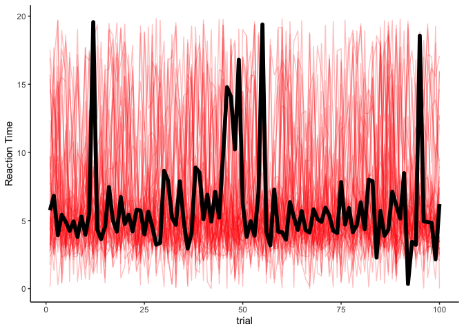
That might appear odd, at first: why do our estimates look the same over time? After the supervised learning, we used the actual latent variables to make predictions of reaction times. But in unsupervised learning, we don’t have access to the latent variables, and so the red lines are just simulated time-series over simulated latent states. You might think that we could use our estimates from the forward algorithm to determine a latent state to simulate from, but that actually poses a problem. Remeber that the forward algorithm generates the joint probability p(zt,y1 : t) . In other words, it produces the joint probability of the data up to time t and the latent state at time t . But what we want is to get the most likely sequence of latent states given the data, p(z1 : t|y1 : t) . To do that, we’ll use the Viterbi algorithm.
The Viterbi algorithm
Whereas the forward algorithm gives us the joint probability of the data up to time t and the latent state at time t , the Viterbi algorithm instead gives us a probability over sequences of latent states given the data. To explain the Viterbi algorithm, let’s look at the Stan code:
1
2
model.viterbi <- cmdstan_model('2022-02-21-hmm2.stan')
model.viterbi
1
2
3
4
5
6
7
8
9
10
11
12
13
14
15
16
17
18
19
20
21
22
23
24
25
26
27
28
29
30
31
32
33
34
35
36
37
38
39
40
41
42
43
44
45
46
47
48
49
50
51
52
53
54
55
56
57
58
59
60
61
62
63
64
65
66
67
68
69
70
71
72
73
74
75
76
77
78
79
80
81
82
83
84
85
86
87
88
89
90
91
92
93
94
95
96
97
98
99
100
101
102
103
104
105
106
107
108
109
110
111
112
113
114
115
116
117
118
119
120
121
122
123
124
125
126
127
128
129
130
131
132
133
134
135
136
137
138
139
140
141
142
143
144
functions {
  // get the log-likelihood of y given z, mu, sigma, and y_max
  real lognormal_mix_lpdf(real y, int z, real mu, real sigma, real y_max) {
    if (z == 1)
      return lognormal_lpdf(y | mu, sigma);
    else
      return uniform_lpdf(y | 0, y_max);
  }

  // simulate y given z, mu, sigma, and y_max
  real lognormal_mix_rng(int z, real mu, real sigma, real y_max) {
    if (z == 1)
      return lognormal_rng(mu, sigma);
    else
      return uniform_rng(0, y_max);
  }

  // forward algorithm for calculating log-likelihood of y
  array[,] real forward(vector y, array[] vector theta, vector pi, real mu, real sigma, real y_max) {
    int N = size(y);
    int K = size(pi);

    array[K] real acc;       // temporary variable
    array[N, K] real alpha;  // log p(y[1:n], z[n]==k)

    // first observation
    for (k in 1:K)
      alpha[1, k] = log(pi[k]) + lognormal_mix_lpdf(y[1] | k, mu, sigma, y_max);

    for (n in 2:N) {
      for (k in 1:K) {
    for (j in 1:K) {
      // calculate log p(y[1:n], z[n]==k, z[n-1]==j)
      acc[j] = alpha[n-1, j] + log(theta[j, k]) +
        lognormal_mix_lpdf(y[n] | k, mu, sigma, y_max);
    }

    alpha[n, k] = log_sum_exp(acc);  // marginalize over all previous states j
      }
    }

    return alpha;
  }

  // viterbi algorithm for finding most likely sequence of latent states given y
  array[] int viterbi(vector y, array[] vector theta, vector pi, real mu, real sigma, real y_max) {
    int N = size(y);
    int K = size(pi);

    array[N] int z_rep;   // simulated latent variables

    // the log probability of the best sequence to state k at time n
    array[N, K] real best_lp = rep_array(negative_infinity(), N, K);

    // the state preceding the current state in the best path
    array[N, K] int back_ptr;

    // first observation
    for (k in 1:K)
      best_lp[1, k] = log(pi[k]) + lognormal_mix_lpdf(y[1] | k, mu, sigma, y_max);

    // for each timepoint n and each state k, find most likely previous state j
    for (n in 2:N) {
      for (k in 1:K) {
        for (j in 1:K) {
      // calculate the log probability of path to k from j
          real lp = best_lp[n-1, j] + log(theta[j, k]) +
        lognormal_mix_lpdf(y[n] | k, mu, sigma, y_max);

          if (lp > best_lp[n, k]) {
            back_ptr[n, k] = j;
            best_lp[n, k] = lp;
          }
        }
      }
    }

    // reconstruct most likely path
    for (k in 1:K)
      if (best_lp[N, k] == max(best_lp[N]))
        z_rep[N] = k;
    for (t in 1:(N - 1))
      z_rep[N - t] = back_ptr[N - t + 1, z_rep[N - t + 1]];

    return z_rep;
  }
}

data {
  int<lower=0> N;                         // number of data points
  vector<lower=0>[N] y;                   // data points
}

transformed data {
  int K = 2;                  // number of latent states (1=attentive, 2=guess)
  real y_max = max(y);        // maximum y value
}

parameters {
  array[K] simplex[K] theta;  // transition matrix

  real mu;                    // lognormal location
  real<lower=0> sigma;        // lognormal scale
}

transformed parameters {
  simplex[K] pi;              // starting probabilities

  {
    // copy theta to a matrix
    matrix[K, K] t;
    for(j in 1:K){
      for(i in 1:K){
    t[i,j] = theta[i,j];
      }
    }

    // solve for pi (assuming pi = pi * theta)
    pi = to_vector((to_row_vector(rep_vector(1.0, K))/
            (diag_matrix(rep_vector(1.0, K)) - t + rep_matrix(1, K, K))));
  }

  array[N, K] real alpha = forward(y, theta, pi, mu, sigma, y_max);
}

model {
  for (k in 1:K)
    theta[k] ~ dirichlet([1, 1]');

  mu ~ std_normal();
  sigma ~ std_normal();

  target += log_sum_exp(alpha[N]);     // marginalize over all ending states
}

generated quantities {
  // Viterbi algorithm
  array[N] int<lower=1, upper=K> z_rep;   // simulated latent variables
  vector<lower=0>[N] y_rep;               // simulated data points

  z_rep = viterbi(y, theta, pi, mu, sigma, y_max);
  for (n in 1:N)
    y_rep[n] = lognormal_mix_rng(z_rep[n], mu, sigma, y_max);
}
In the Viterbi algorithm, we want to estimate the most likely sequence
of latent states
z1 : N
given all of the data y1 : N. So, our first task is to
fill out two matrices. Each element of best_lp[n, k] stores the log
probability of the best path
z1 : n
where
zn = k
. Similarly, each element of back_ptr[n, k] stores the preceding
latent state
zn − 1
so that once we’ve found the best path, we can reconstruct it. The first
set of for loops simply fills out these matrices row by row, finding
the best path up to timepoint
n
. Once we have that, we can use it to find the best path up to the next
timepoint, since in a Markov chain we only need to know about the latent
state one timepoint in the past. Once these matrices are filled out, we
can reconstruct the most likely path starting with timepoint N and
working backwards using our back_ptr. Finally, once we have the
sequence of latent states, we can simulate reaction times as before.
Let’s run the model again and see how it fares:
1
2
fit.viterbi <- model.viterbi$sample(data=list(N=nrow(rts), y=rts$rt))
fit.viterbi$summary(c('theta', 'pi', 'mu', 'sigma'))
1
2
3
4
5
6
7
8
9
10
11
12
13
14
15
16
17
18
19
20
21
22
23
24
25
26
27
28
29
30
31
32
33
34
35
36
37
38
39
40
41
42
43
44
45
46
47
48
49
50
51
52
53
54
55
56
57
58
59
60
61
62
63
64
65
66
67
68
69
70
71
72
73
74
75
76
77
78
79
80
81
82
83
84
85
86
87
88
89
90
91
92
93
94
95
96
97
98
99
100
101
102
103
104
105
106
107
108
109
## Running MCMC with 4 chains, at most 20 in parallel...
##
## Chain 1 Iteration:    1 / 2000 [  0%]  (Warmup)
## Chain 2 Iteration:    1 / 2000 [  0%]  (Warmup)
## Chain 3 Iteration:    1 / 2000 [  0%]  (Warmup)
## Chain 4 Iteration:    1 / 2000 [  0%]  (Warmup)
## Chain 1 Iteration:  100 / 2000 [  5%]  (Warmup)
## Chain 4 Iteration:  100 / 2000 [  5%]  (Warmup)
## Chain 2 Iteration:  100 / 2000 [  5%]  (Warmup)
## Chain 3 Iteration:  100 / 2000 [  5%]  (Warmup)
## Chain 4 Iteration:  200 / 2000 [ 10%]  (Warmup)
## Chain 1 Iteration:  200 / 2000 [ 10%]  (Warmup)
## Chain 3 Iteration:  200 / 2000 [ 10%]  (Warmup)
## Chain 1 Iteration:  300 / 2000 [ 15%]  (Warmup)
## Chain 4 Iteration:  300 / 2000 [ 15%]  (Warmup)
## Chain 2 Iteration:  200 / 2000 [ 10%]  (Warmup)
## Chain 1 Iteration:  400 / 2000 [ 20%]  (Warmup)
## Chain 3 Iteration:  300 / 2000 [ 15%]  (Warmup)
## Chain 4 Iteration:  400 / 2000 [ 20%]  (Warmup)
## Chain 2 Iteration:  300 / 2000 [ 15%]  (Warmup)
## Chain 1 Iteration:  500 / 2000 [ 25%]  (Warmup)
## Chain 3 Iteration:  400 / 2000 [ 20%]  (Warmup)
## Chain 2 Iteration:  400 / 2000 [ 20%]  (Warmup)
## Chain 4 Iteration:  500 / 2000 [ 25%]  (Warmup)
## Chain 1 Iteration:  600 / 2000 [ 30%]  (Warmup)
## Chain 3 Iteration:  500 / 2000 [ 25%]  (Warmup)
## Chain 2 Iteration:  500 / 2000 [ 25%]  (Warmup)
## Chain 4 Iteration:  600 / 2000 [ 30%]  (Warmup)
## Chain 1 Iteration:  700 / 2000 [ 35%]  (Warmup)
## Chain 3 Iteration:  600 / 2000 [ 30%]  (Warmup)
## Chain 4 Iteration:  700 / 2000 [ 35%]  (Warmup)
## Chain 2 Iteration:  600 / 2000 [ 30%]  (Warmup)
## Chain 1 Iteration:  800 / 2000 [ 40%]  (Warmup)
## Chain 3 Iteration:  700 / 2000 [ 35%]  (Warmup)
## Chain 2 Iteration:  700 / 2000 [ 35%]  (Warmup)
## Chain 4 Iteration:  800 / 2000 [ 40%]  (Warmup)
## Chain 1 Iteration:  900 / 2000 [ 45%]  (Warmup)
## Chain 3 Iteration:  800 / 2000 [ 40%]  (Warmup)
## Chain 4 Iteration:  900 / 2000 [ 45%]  (Warmup)
## Chain 2 Iteration:  800 / 2000 [ 40%]  (Warmup)
## Chain 1 Iteration: 1000 / 2000 [ 50%]  (Warmup)
## Chain 1 Iteration: 1001 / 2000 [ 50%]  (Sampling)
## Chain 3 Iteration:  900 / 2000 [ 45%]  (Warmup)
## Chain 2 Iteration:  900 / 2000 [ 45%]  (Warmup)
## Chain 4 Iteration: 1000 / 2000 [ 50%]  (Warmup)
## Chain 4 Iteration: 1001 / 2000 [ 50%]  (Sampling)
## Chain 3 Iteration: 1000 / 2000 [ 50%]  (Warmup)
## Chain 3 Iteration: 1001 / 2000 [ 50%]  (Sampling)
## Chain 1 Iteration: 1100 / 2000 [ 55%]  (Sampling)
## Chain 2 Iteration: 1000 / 2000 [ 50%]  (Warmup)
## Chain 2 Iteration: 1001 / 2000 [ 50%]  (Sampling)
## Chain 4 Iteration: 1100 / 2000 [ 55%]  (Sampling)
## Chain 3 Iteration: 1100 / 2000 [ 55%]  (Sampling)
## Chain 2 Iteration: 1100 / 2000 [ 55%]  (Sampling)
## Chain 1 Iteration: 1200 / 2000 [ 60%]  (Sampling)
## Chain 4 Iteration: 1200 / 2000 [ 60%]  (Sampling)
## Chain 3 Iteration: 1200 / 2000 [ 60%]  (Sampling)
## Chain 1 Iteration: 1300 / 2000 [ 65%]  (Sampling)
## Chain 2 Iteration: 1200 / 2000 [ 60%]  (Sampling)
## Chain 4 Iteration: 1300 / 2000 [ 65%]  (Sampling)
## Chain 3 Iteration: 1300 / 2000 [ 65%]  (Sampling)
## Chain 1 Iteration: 1400 / 2000 [ 70%]  (Sampling)
## Chain 2 Iteration: 1300 / 2000 [ 65%]  (Sampling)
## Chain 4 Iteration: 1400 / 2000 [ 70%]  (Sampling)
## Chain 3 Iteration: 1400 / 2000 [ 70%]  (Sampling)
## Chain 1 Iteration: 1500 / 2000 [ 75%]  (Sampling)
## Chain 2 Iteration: 1400 / 2000 [ 70%]  (Sampling)
## Chain 4 Iteration: 1500 / 2000 [ 75%]  (Sampling)
## Chain 3 Iteration: 1500 / 2000 [ 75%]  (Sampling)
## Chain 1 Iteration: 1600 / 2000 [ 80%]  (Sampling)
## Chain 2 Iteration: 1500 / 2000 [ 75%]  (Sampling)
## Chain 4 Iteration: 1600 / 2000 [ 80%]  (Sampling)
## Chain 3 Iteration: 1600 / 2000 [ 80%]  (Sampling)
## Chain 1 Iteration: 1700 / 2000 [ 85%]  (Sampling)
## Chain 2 Iteration: 1600 / 2000 [ 80%]  (Sampling)
## Chain 4 Iteration: 1700 / 2000 [ 85%]  (Sampling)
## Chain 3 Iteration: 1700 / 2000 [ 85%]  (Sampling)
## Chain 1 Iteration: 1800 / 2000 [ 90%]  (Sampling)
## Chain 4 Iteration: 1800 / 2000 [ 90%]  (Sampling)
## Chain 2 Iteration: 1700 / 2000 [ 85%]  (Sampling)
## Chain 3 Iteration: 1800 / 2000 [ 90%]  (Sampling)
## Chain 1 Iteration: 1900 / 2000 [ 95%]  (Sampling)
## Chain 2 Iteration: 1800 / 2000 [ 90%]  (Sampling)
## Chain 4 Iteration: 1900 / 2000 [ 95%]  (Sampling)
## Chain 3 Iteration: 1900 / 2000 [ 95%]  (Sampling)
## Chain 1 Iteration: 2000 / 2000 [100%]  (Sampling)
## Chain 1 finished in 20.3 seconds.
## Chain 2 Iteration: 1900 / 2000 [ 95%]  (Sampling)
## Chain 4 Iteration: 2000 / 2000 [100%]  (Sampling)
## Chain 4 finished in 20.5 seconds.
## Chain 3 Iteration: 2000 / 2000 [100%]  (Sampling)
## Chain 3 finished in 21.2 seconds.
## Chain 2 Iteration: 2000 / 2000 [100%]  (Sampling)
## Chain 2 finished in 21.6 seconds.
##
## All 4 chains finished successfully.
## Mean chain execution time: 20.9 seconds.
## Total execution time: 21.7 seconds.
## # A tibble: 8 × 10
##   variable    mean median      sd     mad     q5   q95  rhat ess_bulk ess_tail
##   <chr>      <dbl>  <dbl>   <dbl>   <dbl>  <dbl> <dbl> <dbl>    <dbl>    <dbl>
## 1 theta[1,1] 0.897  0.897 0.00966 0.00964 0.880  0.912  1.00    3522.    3167.
## 2 theta[2,1] 0.242  0.241 0.0218  0.0220  0.207  0.278  1.00    3652.    3207.
## 3 theta[1,2] 0.103  0.103 0.00966 0.00964 0.0877 0.120  1.00    3522.    3167.
## 4 theta[2,2] 0.758  0.759 0.0218  0.0220  0.722  0.793  1.00    3652.    3207.
## 5 pi[1]      0.700  0.700 0.0214  0.0216  0.664  0.734  1.00    5367.    3453.
## 6 pi[2]      0.300  0.300 0.0214  0.0216  0.266  0.336  1.00    5367.    3453.
## 7 mu         1.51   1.51  0.00921 0.00910 1.49   1.52   1.00    3841.    3054.
## 8 sigma      0.337  0.337 0.00756 0.00728 0.325  0.349  1.00    3593.    3336.
Once again, the model fit well- this should be no surprise, since we haven’t changed anything about the fitting process (we only changed the way in which we are simulating data). Let’s now see our reconstructed latent states:
1
2
3
4
5
6
7
8
9
10
11
12
13
14
15
16
17
p.model <- fit.viterbi %>%
    spread_draws(z_rep[trial], ndraws=10) %>%
    filter(trial <= 100) %>%
    ggplot(aes(x=trial, y=1-z_rep)) +
    geom_rect(aes(group=.draw, xmin=trial, xmax=trial+1, ymin=0, ymax=1-z_rep), fill='black') +
    facet_grid(.draw ~ .) +
    theme_classic()

(p.data / p.model) +
    plot_layout(heights=c(1, 10)) &
    xlab('Trial') &
    theme(axis.title.y=element_blank(),
          axis.ticks.y=element_blank(),
          axis.text.y=element_blank(),
          axis.line.y=element_blank(),
          strip.background = element_blank(),
          strip.text = element_blank())
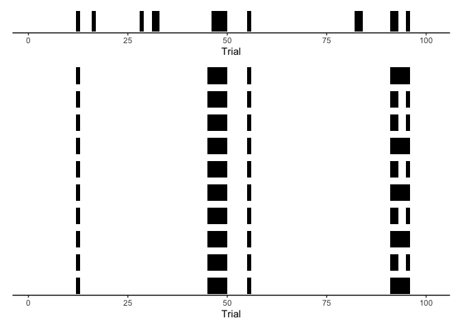
It certainly isn’t perfect, but given that we haven’t observed the latent states we’re in the right ball park. Finally, let’s look at the reconstructed reaction times:
1
2
3
4
5
6
7
fit.viterbi %>%
    spread_draws(y_rep[trial], ndraws=50) %>%
    filter(trial <= 100) %>%
    ggplot(aes(x=trial, y=y_rep)) +
    geom_line(aes(group=.draw), alpha=.25, size=.5, color='red') +
    geom_line(aes(y=rt), data=filter(rts, trial<=100), size=2) +
    theme_classic() + ylab('Reaction Time')
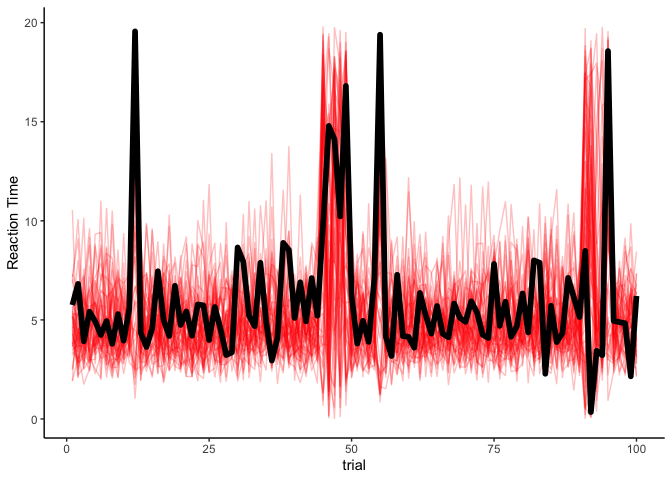
As you can see, these estimates are very comparable to the ones from the supervised learning case! So, even if we haven’t perfectly recovered the sequence of latent states, we seem to be estimating the reaction times just fine. A good explanation for this is that whenever we are missing periods of inattention, it is because the reaction times during those periods look similar to reaction times during attention, and since participants are more attentive than not, those reaction times are well-explained as if they were coming from an attentive state.
Conclusions
We’ve covered a lot in this tutorial: from building a simple reaction time model, enhancing it to model random responses during inattention, and using HMMs to model the dynamics of attention during psychological tasks, and fitting the HMM in a supervised and unsupervised manner. However, there’s always much more that can be done. Similar to mixed-effects regression, hierarchical HMMs model participant-level (or item-level, etc) trends in latent dynamics and responses. It is also common to model effects on the transition matrices or mixture distributions as a function of covariates like age or gender. No matter what direction you’re heading, hopefully this tutorial provided a good foundation to start.