Intro to Probabilistic Programming with Stan
In this tutorial we’re going to talk about what probabilistic programming is and how we can use it for statistical modeling. If you aren’t familiar at all with Bayesian stats, check out my previous post on the topic. If you’re used to probabilistic programming but just want to learn the Stan language, you can go straight to the fantastic Stan User’s Guide, which explains how to program a wide variety of models.
- What is probabilistic programming?
- Probabilistic programming with Stan
- Assessing model convergence
- Assessing model fit
- Linear Regression in Stan
- Summary
What is probabilistic programming?
Probabilistic programming is a relatively new and exciting approach to statistical modeling that lets you create models in a standardized language without having to implement any of the nitty-gritty details or work out too much math. Although not all probabilistic programs are Bayesian, probabalistic programming makes Bayesian modeling easy, and so it’s a great way to learn what Bayesian models are, how they’re fit to data, and what you can do with them. To explain what probabilistic programming is, I’m going to use just a little bit of math. Bear with me, because this is important!
In Bayesian statistics, we start with a model and some data. As a simple example, we might model some ratings on a scale using a normal distribution with a particular mean μ and variance σ2 . Our goal is to identify the most likely parameter values given our data (that is, the values of μ and σ that best explain our data). To determine which which parameter values are best, we make use of Bayes’ formula:
P(θ|𝒟) ∝ P(θ)P(𝒟|θ)
This formula says that the probability of a parameter value θ given our data 𝒟 is proportional to our prior probability of that parameter value multiplied by the likelihood that the data could have been generated from that parameter value. How do we determine the likelihood? Well, sometimes we can derive the likelihood (and hence the posterior) by hand. But in most cases, this approach is too difficult or time-consuming. In probabilistic programming, we write a program that simulates our model given some parameter values. This is actually useful in its own right: we can use this program to see how the model behaves under different settings of the parameters. But in statistical inference, the important part is that we run that program to (approximately) calculate the likelihood, which in turn lets us calculate the posterior probability of the parameter values given our data.
Why Stan?
There are a good number of probabilistic programming languages out
there. Today we’re going to focus on Stan, which
is one of the fastest, most reliable, and most widely used probabilistic
programming languages out there. One of the cool things about Stan is
that there are a number of different interfactes to Stan: you can use
Stan through R, through Python, through Matlab, through Julia, and even
directly through the command-line! If you’ve read my tutorial on
Bayesian regression with
brms, then you’ve
actually already used one of the easiest interfaces to Stan, which
writes Stan programs for you based on lmer-like formulas. Lastly, Stan
has one of the largest communities
that makes getting coding help and statistical advice easy.
The components of a Stan program
Unsurprisingly, Stan programs are written in Stan files, which use the
extension .stan. The Stan language has similar syntax to C++, in
that it uses curly braces ({ and }) to define blocks of code,
semicolons (;) after each statement, and has a type declaration for
every variable in the program. There are two primitive data types: int
for integers, and real for floating-point/decimal numbers. There are
also a few different container types: array, vector, and
row_vector for one-dimensional containers, and matrix for
N-dimensional containers. For now, the differences between array,
vector, and row_vector aren’t that important. Just know that when
possible, we will try to use type vector, which will generally be most
efficient.
Stan programs consist of up to seven different blocks of code, in the following order (*required):
functionsdata*transformed dataparameters*transformed parametersmodel*generated quantities
In the remainder of the workshop, we’re going to focus on the data,
parameters, model, and generated_quantities blocks, but we’ll also
use the transformed parameters block.
Probabilistic programming with Stan
To demonstrate the power of Stan, let’s first get a nice dataset to work with. Here I’m going to load some packages, and then run some code to gather data from the Spotify top 200 songs per week in 2021. Don’t worry about how this code actually works (we can save that for a future meeting…), but know that it will take some time (~5mins) if you run this on your computer.
Getting some data
1
2
3
4
5
6
7
8
9
10
11
12
13
14
15
16
17
18
19
20
21
22
23
24
25
26
27
28
29
30
31
32
33
34
35
36
37
38
39
40
41
42
43
44
45
46
47
48
49
50
51
52
53
54
55
56
57
58
59
60
61
62
63
library(cmdstanr)   # for stan
library(tidyverse)  # for data wrangling
library(lubridate)  # for dates
library(rvest)      # for scraping spotify charts
library(spotifyr)   # for spotify audio features
library(tidybayes)  # for accessing model posteriors
library(viridis)    # for pretty plots
options(mc.cores=parallel::detectCores())

## gather spotify chart data (modified from https://rpubs.com/argdata/web_scraping)
scrape_spotify <- function(url) {
    page <- url %>% read_html() # read the HTML page

    rank <- page %>%
        html_elements('.chart-table-position') %>%
        html_text() %>%
        as.integer
    track <- page %>%
        html_elements('strong') %>%
        html_text()
    artist <- page %>%
        html_elements('.chart-table-track span') %>%
        html_text() %>%
        str_remove('by ')
    streams <- page %>%
        html_elements('td.chart-table-streams') %>%
        html_text() %>%
        str_remove_all(',') %>%
        as.integer
    URI <- page %>%
        html_elements('a') %>%
        html_attr('href') %>%
        str_subset('https://open.spotify.com/track/') %>%
        str_remove('https://open.spotify.com/track/')

    ## combine, name, and make it a tibble
    chart <- tibble(rank=rank, track=track, artist=artist, streams=streams, URI=URI)
    return(chart)
}

## setup access to Spotify API
access_token <- get_spotify_access_token()

## load the top 200 songs in the US per week in 2021
spotify2021 <- tibble(week=seq(ymd('2021-01-01'), ymd('2021-11-19'), by = 'weeks')) %>%
    mutate(url=paste0('https://spotifycharts.com/regional/us/weekly/', week, '--', week+days(7)),
           data=map(url, scrape_spotify)) %>%
    unnest(data) %>%
    mutate(streams=streams/1000000)

## extract spotify's audio features for each song
features <- tibble(URI=unique(spotify2021$URI)) %>%
    mutate(features=map(URI, ~ get_track_audio_features(.x, authorization=access_token))) %>%
    unnest(features)

## make one tidy data frame
spotify2021 <- spotify2021 %>% left_join(features, by='URI') %>%
    select(-URI, -analysis_url, -track_href, -id, -type) %>%
    relocate(week, rank, track, artist, streams, duration_ms, tempo,
             time_signature, key, mode, valence, loudness, danceability,
             energy, speechiness, acousticness, instrumentalness, liveness, uri, url)
write_csv(spotify2021, '2021-12-10-spotify-data.csv')
spotify2021
1
2
3
4
5
6
7
8
9
10
11
12
13
14
15
16
17
## # A tibble: 9,400 × 20
##    week        rank track  artist streams duration_ms tempo time_signature   key
##    <date>     <dbl> <chr>  <chr>    <dbl>       <dbl> <dbl>          <dbl> <dbl>
##  1 2021-01-01     1 Good … SZA       6.32      279204 121.               4     1
##  2 2021-01-01     2 Anyone Justi…    6.15      190779 116.               4     2
##  3 2021-01-01     3 34+35  Arian…    5.61      173711 110.               4     0
##  4 2021-01-01     4 Mood … 24kGo…    5.58      140526  91.0              4     7
##  5 2021-01-01     5 Lemon… Inter…    5.37      195429 140.               4     1
##  6 2021-01-01     6 DÁKITI Bad B…    5.16      205090 110.               4     4
##  7 2021-01-01     7 posit… Arian…    5.10      172325 144.               4     0
##  8 2021-01-01     8 Whoop… CJ        4.88      123263 140.               4     3
##  9 2021-01-01     9 WITHO… The K…    4.78      161385  93.0              4     0
## 10 2021-01-01    10 Blind… The W…    4.44      200040 171.               4     1
## # … with 9,390 more rows, and 11 more variables: mode <dbl>, valence <dbl>,
## #   loudness <dbl>, danceability <dbl>, energy <dbl>, speechiness <dbl>,
## #   acousticness <dbl>, instrumentalness <dbl>, liveness <dbl>, uri <chr>,
## #   url <chr>
As we can see, we now have a dataframe of Spotify’s weekly top 200 tracks, along with the following information:
week: the week in 2021rank: the song’s rank (1to200) in this week, with1being the top songtrack: the name of the songartist: the name of the artist who released the songstreams: the number of streams in that week (in millions)duration_ms: the duration of the track in mstempo: the tempo of the track in beats per minutetime_signature: an estimated time signature ranging from3to7(for 3/4 to 7/4)key: the key of the song from0(for C) to11(for B), or-1if no key was foundmode: whether the track is in a major (1) or minor (0) keyvalence: the emotional valence of the track from0(negative valence/sad) to1(positive valence/happy)loudness: the average loudness of the track in decibelsdanceability: an estimate of how danceable the track is, from0(least danceable) to1(most danceable)energy: an estimate of the intensity or activity of the track, from0(low energy) to1(high energy)speechiness: an estimate of the proportion of speech in the track, from0(no speech) to1(only speech)acousticness: an estimate of the degree to which a track is (1) or is not (0) acousticinstrumentalness: an estimate of the degree to which a track contains (1) or does not contain (0) vocalsliveness: an estimate of whether the track was performed live (1) or not (0)uri: the Spotify unique identifier for the trackurl: a link to the track
Simulating fake data: number of streams
Let’s say we want to know how many times, on average, the top 200 tracks
are streamed every week. Of course, we could just use
mean(spotify2021$streams) to get this number, but to get more
information we will need to specify a model. As a start, we can assume a
normal distribution with mean
μ
and standard deviation
σ
. Before fitting this model, we might just want to know what data
simulated from this model looks like under different parameter values.
This is the main goal of simulation: we assume that we know what the
values of
μ
and
σ
are to check what the distribution of streams would look like if those
values were true. To do that, let’s write a Stan program, which I’ll
save in the file 2021-12-10-streams-sim.stan:
1
2
3
4
5
6
7
8
9
10
11
12
13
14
15
data {
  real<lower=0> mu;       // the mean
  real<lower=0> sigma;    // the standard deviation
}

parameters {
}

model {
}

generated quantities {
  // simulate data using a normal distribution
  real y_hat = normal_rng(mu, sigma);
}
Since we’re simulating from a prior, we will take our parameters mu
and sigma as inputs to Stan by declaring them in the data block. The
code real<lower=0> mu; defines a variable called mu that will refer
to the mean of the number of streams, and similarly
real<lower=0> sigma; defines the standard deviation. Both of these
variables are lower-bounded at 0 with the expression <lower=0>,
because it wouldn’t make sense to simulate a negative number of streams
or a negative standard deviation (we would also put an upper bound here
if it made sense). Since our model has no remaining parameters, and we
are not yet modeling any data, both the parameters and model blocks
are empty. Finally, in the generated quantities block, we are telling
our model to simulate the number of streams by drawing a random number
from a normal distribution.
To run our Stan program, we will make use of the library cmdstanr. The
rstan library also works for this, but I’ve found cmdstanr to be
faster and more reliable. Let’s say we know that there are roughly one
million streams per week, but this varies with a standard deviation of
one hundred thousand streams. We can make a list of these values, and
pass them to Stan as data:
1
2
3
streams_sim_data <- list(mu=1, sigma=.1)
streams_sim_model <- cmdstan_model('2021-12-10-streams-sim.stan')  ## compile the model
streams_sim <- streams_sim_model$sample(data=streams_sim_data, fixed_param=TRUE)
1
2
3
4
5
6
7
8
9
10
11
12
13
14
15
16
17
18
19
20
21
22
23
24
25
26
27
28
29
30
31
32
33
34
35
36
37
38
39
40
41
42
43
44
45
46
47
48
49
50
51
52
53
54
## Running MCMC with 4 chains, at most 20 in parallel...
##
## Chain 1 Iteration:   1 / 1000 [  0%]  (Sampling)
## Chain 1 Iteration: 100 / 1000 [ 10%]  (Sampling)
## Chain 1 Iteration: 200 / 1000 [ 20%]  (Sampling)
## Chain 1 Iteration: 300 / 1000 [ 30%]  (Sampling)
## Chain 1 Iteration: 400 / 1000 [ 40%]  (Sampling)
## Chain 1 Iteration: 500 / 1000 [ 50%]  (Sampling)
## Chain 1 Iteration: 600 / 1000 [ 60%]  (Sampling)
## Chain 1 Iteration: 700 / 1000 [ 70%]  (Sampling)
## Chain 1 Iteration: 800 / 1000 [ 80%]  (Sampling)
## Chain 1 Iteration: 900 / 1000 [ 90%]  (Sampling)
## Chain 1 Iteration: 1000 / 1000 [100%]  (Sampling)
## Chain 2 Iteration:   1 / 1000 [  0%]  (Sampling)
## Chain 2 Iteration: 100 / 1000 [ 10%]  (Sampling)
## Chain 2 Iteration: 200 / 1000 [ 20%]  (Sampling)
## Chain 2 Iteration: 300 / 1000 [ 30%]  (Sampling)
## Chain 2 Iteration: 400 / 1000 [ 40%]  (Sampling)
## Chain 2 Iteration: 500 / 1000 [ 50%]  (Sampling)
## Chain 2 Iteration: 600 / 1000 [ 60%]  (Sampling)
## Chain 2 Iteration: 700 / 1000 [ 70%]  (Sampling)
## Chain 2 Iteration: 800 / 1000 [ 80%]  (Sampling)
## Chain 2 Iteration: 900 / 1000 [ 90%]  (Sampling)
## Chain 2 Iteration: 1000 / 1000 [100%]  (Sampling)
## Chain 3 Iteration:   1 / 1000 [  0%]  (Sampling)
## Chain 3 Iteration: 100 / 1000 [ 10%]  (Sampling)
## Chain 3 Iteration: 200 / 1000 [ 20%]  (Sampling)
## Chain 3 Iteration: 300 / 1000 [ 30%]  (Sampling)
## Chain 3 Iteration: 400 / 1000 [ 40%]  (Sampling)
## Chain 3 Iteration: 500 / 1000 [ 50%]  (Sampling)
## Chain 3 Iteration: 600 / 1000 [ 60%]  (Sampling)
## Chain 3 Iteration: 700 / 1000 [ 70%]  (Sampling)
## Chain 3 Iteration: 800 / 1000 [ 80%]  (Sampling)
## Chain 3 Iteration: 900 / 1000 [ 90%]  (Sampling)
## Chain 3 Iteration: 1000 / 1000 [100%]  (Sampling)
## Chain 4 Iteration:   1 / 1000 [  0%]  (Sampling)
## Chain 4 Iteration: 100 / 1000 [ 10%]  (Sampling)
## Chain 4 Iteration: 200 / 1000 [ 20%]  (Sampling)
## Chain 4 Iteration: 300 / 1000 [ 30%]  (Sampling)
## Chain 4 Iteration: 400 / 1000 [ 40%]  (Sampling)
## Chain 4 Iteration: 500 / 1000 [ 50%]  (Sampling)
## Chain 4 Iteration: 600 / 1000 [ 60%]  (Sampling)
## Chain 4 Iteration: 700 / 1000 [ 70%]  (Sampling)
## Chain 4 Iteration: 800 / 1000 [ 80%]  (Sampling)
## Chain 4 Iteration: 900 / 1000 [ 90%]  (Sampling)
## Chain 4 Iteration: 1000 / 1000 [100%]  (Sampling)
## Chain 1 finished in 0.0 seconds.
## Chain 2 finished in 0.0 seconds.
## Chain 3 finished in 0.0 seconds.
## Chain 4 finished in 0.0 seconds.
##
## All 4 chains finished successfully.
## Mean chain execution time: 0.0 seconds.
## Total execution time: 0.3 seconds.
As we can see, the model has simulated 1000 stream counts in four
different chains. Note that above, we used the argument
fixed_param=TRUE to tell Stan that our model has no parameters, which
makes the sampling faster. Let’s look at a summary of our model:
1
streams_sim
1
2
##  variable mean median   sd  mad   q5  q95 rhat ess_bulk ess_tail
##     y_hat 1.00   1.00 0.10 0.10 0.83 1.17 1.00     3848     3898
This summary tells us that our simulated streams counts have an average
of about one million and a standard deviation of about one hundred
thousand. To access the simulated data, we have a few different options.
Within cmdstanr, the default is to use streams_sim$draws(). However,
I find that the spread_draws function from tidybayes is usually
easier to work with, as it gives us a nice tidy dataframe of whatever
variables we want. The other reason is that we’re going to use
tidybayes (technically ggdist) to make pretty plots of our draws.
Let’s get our draws and plot them:
1
2
3
4
5
6
7
draws <- streams_sim %>% gather_draws(y_hat)

ggplot(draws, aes(x=.value)) +
    stat_halfeye(point_interval=median_hdi, normalize='panels') +
    xlab('Streams (millions/week)') + ylab('Density') +
    facet_wrap(~ .variable, scales='free') +
    theme_tidybayes()
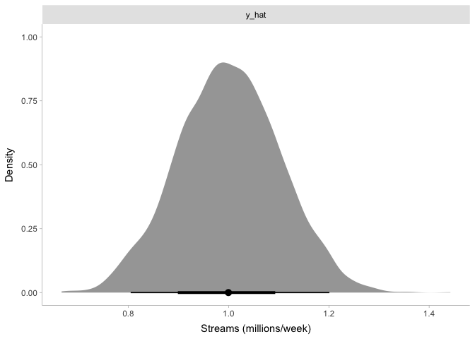
Again, this tells us what we already expected: our simulated top 200 songs have somewhere around one million streams per week, and the number of streams are normally distributed around that.
Sampling from a prior distribution
It’s nice to simulate data, but of course our main goal is to infer what
the actual mean and standard deviation of stream counts for the top
200 tracks. To do so, we first need to define a prior distribution.
Thankfully, this is pretty easy in Stan: we just move the parameters
mu and sigma from the data block to the parameters block:
1
2
3
4
5
6
7
8
9
10
11
12
13
14
15
16
17
18
19
data {

}

parameters {
  real<lower=0> mu;     // the mean
  real<lower=0> sigma;  // the standard deviation
}

model {
  // define priors for mu and sigma
  mu ~ normal(1, .1);
  sigma ~ normal(0, .1);
}

generated quantities {
  // simulate data using a normal distribution
  real y_hat = normal_rng(mu, sigma);
}
Besides the declarations of mu and sigma being moved to the
parameters block, we can see that we’ve also added to the model
block. Specifically, the model block now specifies prior distributions
over our two parameters. The symbol ~ can be read as “is distributed
as”, so we’re saying that mu is distributed according to a normal
distribution with a mean of one million and a standard deviation of one
hundred thousand. Likewise, we’re assuming that sigma is distributed
normally around 0 with a standard deviation of one hundred thousand. You
might think that this would give us negative numbers, but Stan truncates
these normal distributions at 0 because of the <lower=0> in the
paramters’ declarations. Now let’s sample from our prior distribution to
simulate some fake data:
1
2
3
4
5
6
7
8
9
10
11
12
streams_prior_model <- cmdstan_model('2021-12-10-streams-prior.stan')  ## compile the model
streams_prior <- streams_prior_model$sample()
streams_prior

streams_prior %>%
    gather_draws(mu, sigma, y_hat) %>%
    mutate(.variable=factor(.variable, levels=c('y_hat', 'sigma', 'mu'))) %>%
    ggplot(aes(x=.value, y=.variable)) +
    stat_halfeye(point_interval=median_hdi, normalize='panels') +
    xlab('Streams (millions/week)') + ylab('Density') +
    facet_wrap(~ .variable, scales='free') +
    theme_tidybayes()
1
2
3
4
5
6
7
8
9
10
11
12
13
14
15
16
17
18
19
20
21
22
23
24
25
26
27
28
29
30
31
32
33
34
35
36
37
38
39
40
41
42
43
44
45
46
47
48
49
50
51
52
53
54
55
56
57
58
59
60
61
62
63
64
65
66
67
68
69
70
71
72
73
74
75
76
77
78
79
80
81
82
83
84
85
86
87
88
89
90
91
92
93
94
95
96
97
98
99
100
101
102
103
## Running MCMC with 4 chains, at most 20 in parallel...
##
## Chain 1 Iteration:    1 / 2000 [  0%]  (Warmup)
## Chain 1 Iteration:  100 / 2000 [  5%]  (Warmup)
## Chain 1 Iteration:  200 / 2000 [ 10%]  (Warmup)
## Chain 1 Iteration:  300 / 2000 [ 15%]  (Warmup)
## Chain 1 Iteration:  400 / 2000 [ 20%]  (Warmup)
## Chain 1 Iteration:  500 / 2000 [ 25%]  (Warmup)
## Chain 1 Iteration:  600 / 2000 [ 30%]  (Warmup)
## Chain 1 Iteration:  700 / 2000 [ 35%]  (Warmup)
## Chain 1 Iteration:  800 / 2000 [ 40%]  (Warmup)
## Chain 1 Iteration:  900 / 2000 [ 45%]  (Warmup)
## Chain 1 Iteration: 1000 / 2000 [ 50%]  (Warmup)
## Chain 1 Iteration: 1001 / 2000 [ 50%]  (Sampling)
## Chain 1 Iteration: 1100 / 2000 [ 55%]  (Sampling)
## Chain 1 Iteration: 1200 / 2000 [ 60%]  (Sampling)
## Chain 1 Iteration: 1300 / 2000 [ 65%]  (Sampling)
## Chain 1 Iteration: 1400 / 2000 [ 70%]  (Sampling)
## Chain 1 Iteration: 1500 / 2000 [ 75%]  (Sampling)
## Chain 1 Iteration: 1600 / 2000 [ 80%]  (Sampling)
## Chain 1 Iteration: 1700 / 2000 [ 85%]  (Sampling)
## Chain 1 Iteration: 1800 / 2000 [ 90%]  (Sampling)
## Chain 1 Iteration: 1900 / 2000 [ 95%]  (Sampling)
## Chain 1 Iteration: 2000 / 2000 [100%]  (Sampling)
## Chain 2 Iteration:    1 / 2000 [  0%]  (Warmup)
## Chain 2 Iteration:  100 / 2000 [  5%]  (Warmup)
## Chain 2 Iteration:  200 / 2000 [ 10%]  (Warmup)
## Chain 2 Iteration:  300 / 2000 [ 15%]  (Warmup)
## Chain 2 Iteration:  400 / 2000 [ 20%]  (Warmup)
## Chain 2 Iteration:  500 / 2000 [ 25%]  (Warmup)
## Chain 2 Iteration:  600 / 2000 [ 30%]  (Warmup)
## Chain 2 Iteration:  700 / 2000 [ 35%]  (Warmup)
## Chain 2 Iteration:  800 / 2000 [ 40%]  (Warmup)
## Chain 2 Iteration:  900 / 2000 [ 45%]  (Warmup)
## Chain 2 Iteration: 1000 / 2000 [ 50%]  (Warmup)
## Chain 2 Iteration: 1001 / 2000 [ 50%]  (Sampling)
## Chain 2 Iteration: 1100 / 2000 [ 55%]  (Sampling)
## Chain 2 Iteration: 1200 / 2000 [ 60%]  (Sampling)
## Chain 2 Iteration: 1300 / 2000 [ 65%]  (Sampling)
## Chain 2 Iteration: 1400 / 2000 [ 70%]  (Sampling)
## Chain 2 Iteration: 1500 / 2000 [ 75%]  (Sampling)
## Chain 2 Iteration: 1600 / 2000 [ 80%]  (Sampling)
## Chain 2 Iteration: 1700 / 2000 [ 85%]  (Sampling)
## Chain 2 Iteration: 1800 / 2000 [ 90%]  (Sampling)
## Chain 2 Iteration: 1900 / 2000 [ 95%]  (Sampling)
## Chain 2 Iteration: 2000 / 2000 [100%]  (Sampling)
## Chain 3 Iteration:    1 / 2000 [  0%]  (Warmup)
## Chain 3 Iteration:  100 / 2000 [  5%]  (Warmup)
## Chain 3 Iteration:  200 / 2000 [ 10%]  (Warmup)
## Chain 3 Iteration:  300 / 2000 [ 15%]  (Warmup)
## Chain 3 Iteration:  400 / 2000 [ 20%]  (Warmup)
## Chain 3 Iteration:  500 / 2000 [ 25%]  (Warmup)
## Chain 3 Iteration:  600 / 2000 [ 30%]  (Warmup)
## Chain 3 Iteration:  700 / 2000 [ 35%]  (Warmup)
## Chain 3 Iteration:  800 / 2000 [ 40%]  (Warmup)
## Chain 3 Iteration:  900 / 2000 [ 45%]  (Warmup)
## Chain 3 Iteration: 1000 / 2000 [ 50%]  (Warmup)
## Chain 3 Iteration: 1001 / 2000 [ 50%]  (Sampling)
## Chain 3 Iteration: 1100 / 2000 [ 55%]  (Sampling)
## Chain 3 Iteration: 1200 / 2000 [ 60%]  (Sampling)
## Chain 3 Iteration: 1300 / 2000 [ 65%]  (Sampling)
## Chain 3 Iteration: 1400 / 2000 [ 70%]  (Sampling)
## Chain 3 Iteration: 1500 / 2000 [ 75%]  (Sampling)
## Chain 3 Iteration: 1600 / 2000 [ 80%]  (Sampling)
## Chain 3 Iteration: 1700 / 2000 [ 85%]  (Sampling)
## Chain 3 Iteration: 1800 / 2000 [ 90%]  (Sampling)
## Chain 3 Iteration: 1900 / 2000 [ 95%]  (Sampling)
## Chain 3 Iteration: 2000 / 2000 [100%]  (Sampling)
## Chain 4 Iteration:    1 / 2000 [  0%]  (Warmup)
## Chain 4 Iteration:  100 / 2000 [  5%]  (Warmup)
## Chain 4 Iteration:  200 / 2000 [ 10%]  (Warmup)
## Chain 4 Iteration:  300 / 2000 [ 15%]  (Warmup)
## Chain 4 Iteration:  400 / 2000 [ 20%]  (Warmup)
## Chain 4 Iteration:  500 / 2000 [ 25%]  (Warmup)
## Chain 4 Iteration:  600 / 2000 [ 30%]  (Warmup)
## Chain 4 Iteration:  700 / 2000 [ 35%]  (Warmup)
## Chain 4 Iteration:  800 / 2000 [ 40%]  (Warmup)
## Chain 4 Iteration:  900 / 2000 [ 45%]  (Warmup)
## Chain 4 Iteration: 1000 / 2000 [ 50%]  (Warmup)
## Chain 4 Iteration: 1001 / 2000 [ 50%]  (Sampling)
## Chain 4 Iteration: 1100 / 2000 [ 55%]  (Sampling)
## Chain 4 Iteration: 1200 / 2000 [ 60%]  (Sampling)
## Chain 4 Iteration: 1300 / 2000 [ 65%]  (Sampling)
## Chain 4 Iteration: 1400 / 2000 [ 70%]  (Sampling)
## Chain 4 Iteration: 1500 / 2000 [ 75%]  (Sampling)
## Chain 4 Iteration: 1600 / 2000 [ 80%]  (Sampling)
## Chain 4 Iteration: 1700 / 2000 [ 85%]  (Sampling)
## Chain 4 Iteration: 1800 / 2000 [ 90%]  (Sampling)
## Chain 4 Iteration: 1900 / 2000 [ 95%]  (Sampling)
## Chain 4 Iteration: 2000 / 2000 [100%]  (Sampling)
## Chain 1 finished in 0.0 seconds.
## Chain 2 finished in 0.0 seconds.
## Chain 3 finished in 0.0 seconds.
## Chain 4 finished in 0.0 seconds.
##
## All 4 chains finished successfully.
## Mean chain execution time: 0.0 seconds.
## Total execution time: 0.2 seconds.
##  variable  mean median   sd  mad    q5   q95 rhat ess_bulk ess_tail
##     lp__  -3.94  -3.61 1.08 0.83 -6.10 -2.85 1.00     1430     1617
##     mu     1.00   1.00 0.10 0.10  0.84  1.17 1.00     1960     1705
##     sigma  0.08   0.07 0.06 0.06  0.01  0.20 1.00     1391     1210
##     y_hat  1.00   1.00 0.14 0.13  0.78  1.24 1.00     2721     2915
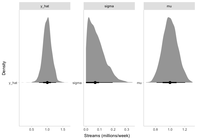
Just like before, we now have simulated values of y_hat centered
around one million streams per week. However, the distribution of
y_hat is wider than before. When we simulated stream counts with a
fixed mu and sigma, the only source of noise in our simulated data
was the noise in the sampling process. But now that we have included
mu and sigma as parameters in the model, we also have uncertainty in
mu and sigma that creates some more noise in y_hat.
Fitting a model to data
You might have noticed that that was a whole lot of work to go through
to sample from some normal distributions. Up until now, we could have
just as well used rnorm a few times to do the trick. So what’s the
point? Well, using (almost) the same Stan code, we can now fit this
simple model to our data to find the most likely values of
μ
and
σ
:
1
2
3
4
5
6
7
8
9
10
11
12
13
14
15
16
17
18
19
20
21
22
23
data {
  int<lower=0> N;         // the number of data points
  vector<lower=0>[N] y;   // the data to model
}

parameters {
  real<lower=0> mu;       // the mean
  real<lower=0> sigma;    // the standard deviation
}

model {
  // define priors for mu and sigma
  mu ~ normal(1, .1);
  sigma ~ normal(0, .1);

  // define the likelihood of y
  y ~ normal(mu, sigma);
}

generated quantities {
  // simulate data using a normal distribution
  real y_hat = normal_rng(mu, sigma);
}
Compared to the previous code, we have added two things. First, in the
data block, we added declarations for two variables. y is a vector
containing the stream counts for each track in each week. The syntax
[N] tells Stan that this vector is N numbers long, which is why we
also declared a data variable N. Finally, in the model block, we
added a line that defines the likelihood of y given our model: we are
modeling y as normally-distributed with mean mu and standard
deviation sigma. Rather than just evaluating the likelihood of the
data according to our prior distributions, Stan will sample the values
of mu and sigma according to their posterior probability using
Markov Chain Monte Carlo (MCMC), giving us an approximate posterior
distribution. Let’s run it and see what happens:
1
2
3
4
5
6
7
8
9
10
11
streams_data <- list(N=nrow(spotify2021), y=spotify2021$streams)
streams_model <- cmdstan_model('2021-12-10-streams.stan')  ## compile the model
streams <- streams_model$sample(data=streams_data, save_warmup=TRUE)
streams

draws <- streams %>% gather_draws(mu, sigma, y_hat)
ggplot(draws, aes(x=.value)) +
    stat_halfeye(point_interval=median_hdi, normalize='panels') +
    xlab('Streams (millions/week)') + ylab('Density') +
    facet_wrap(~ .variable, scales='free') +
    theme_tidybayes()
1
2
3
4
5
6
7
8
9
10
11
12
13
14
15
16
17
18
19
20
21
22
23
24
25
26
27
28
29
30
31
32
33
34
35
36
37
38
39
40
41
42
43
44
45
46
47
48
49
50
51
52
53
54
55
56
57
58
59
60
61
62
63
64
65
66
67
68
69
70
71
72
73
74
75
76
77
78
79
80
81
82
83
84
85
86
87
88
89
90
91
92
93
94
95
96
97
98
99
100
101
102
103
104
105
106
107
108
## Running MCMC with 4 chains, at most 20 in parallel...
##
## Chain 1 Iteration:    1 / 2000 [  0%]  (Warmup)
## Chain 1 Iteration:  100 / 2000 [  5%]  (Warmup)
## Chain 1 Iteration:  200 / 2000 [ 10%]  (Warmup)
## Chain 1 Iteration:  300 / 2000 [ 15%]  (Warmup)
## Chain 1 Iteration:  400 / 2000 [ 20%]  (Warmup)
## Chain 1 Iteration:  500 / 2000 [ 25%]  (Warmup)
## Chain 1 Iteration:  600 / 2000 [ 30%]  (Warmup)
## Chain 1 Iteration:  700 / 2000 [ 35%]  (Warmup)
## Chain 1 Iteration:  800 / 2000 [ 40%]  (Warmup)
## Chain 1 Iteration:  900 / 2000 [ 45%]  (Warmup)
## Chain 1 Iteration: 1000 / 2000 [ 50%]  (Warmup)
## Chain 1 Iteration: 1001 / 2000 [ 50%]  (Sampling)
## Chain 1 Iteration: 1100 / 2000 [ 55%]  (Sampling)
## Chain 1 Iteration: 1200 / 2000 [ 60%]  (Sampling)
## Chain 2 Iteration:    1 / 2000 [  0%]  (Warmup)
## Chain 2 Iteration:  100 / 2000 [  5%]  (Warmup)
## Chain 2 Iteration:  200 / 2000 [ 10%]  (Warmup)
## Chain 2 Iteration:  300 / 2000 [ 15%]  (Warmup)
## Chain 2 Iteration:  400 / 2000 [ 20%]  (Warmup)
## Chain 2 Iteration:  500 / 2000 [ 25%]  (Warmup)
## Chain 2 Iteration:  600 / 2000 [ 30%]  (Warmup)
## Chain 2 Iteration:  700 / 2000 [ 35%]  (Warmup)
## Chain 2 Iteration:  800 / 2000 [ 40%]  (Warmup)
## Chain 2 Iteration:  900 / 2000 [ 45%]  (Warmup)
## Chain 2 Iteration: 1000 / 2000 [ 50%]  (Warmup)
## Chain 2 Iteration: 1001 / 2000 [ 50%]  (Sampling)
## Chain 2 Iteration: 1100 / 2000 [ 55%]  (Sampling)
## Chain 2 Iteration: 1200 / 2000 [ 60%]  (Sampling)
## Chain 2 Iteration: 1300 / 2000 [ 65%]  (Sampling)
## Chain 2 Iteration: 1400 / 2000 [ 70%]  (Sampling)
## Chain 2 Iteration: 1500 / 2000 [ 75%]  (Sampling)
## Chain 2 Iteration: 1600 / 2000 [ 80%]  (Sampling)
## Chain 2 Iteration: 1700 / 2000 [ 85%]  (Sampling)
## Chain 2 Iteration: 1800 / 2000 [ 90%]  (Sampling)
## Chain 2 Iteration: 1900 / 2000 [ 95%]  (Sampling)
## Chain 2 Iteration: 2000 / 2000 [100%]  (Sampling)
## Chain 3 Iteration:    1 / 2000 [  0%]  (Warmup)
## Chain 3 Iteration:  100 / 2000 [  5%]  (Warmup)
## Chain 3 Iteration:  200 / 2000 [ 10%]  (Warmup)
## Chain 3 Iteration:  300 / 2000 [ 15%]  (Warmup)
## Chain 3 Iteration:  400 / 2000 [ 20%]  (Warmup)
## Chain 3 Iteration:  500 / 2000 [ 25%]  (Warmup)
## Chain 3 Iteration:  600 / 2000 [ 30%]  (Warmup)
## Chain 3 Iteration:  700 / 2000 [ 35%]  (Warmup)
## Chain 3 Iteration:  800 / 2000 [ 40%]  (Warmup)
## Chain 3 Iteration:  900 / 2000 [ 45%]  (Warmup)
## Chain 3 Iteration: 1000 / 2000 [ 50%]  (Warmup)
## Chain 3 Iteration: 1001 / 2000 [ 50%]  (Sampling)
## Chain 3 Iteration: 1100 / 2000 [ 55%]  (Sampling)
## Chain 3 Iteration: 1200 / 2000 [ 60%]  (Sampling)
## Chain 3 Iteration: 1300 / 2000 [ 65%]  (Sampling)
## Chain 3 Iteration: 1400 / 2000 [ 70%]  (Sampling)
## Chain 3 Iteration: 1500 / 2000 [ 75%]  (Sampling)
## Chain 3 Iteration: 1600 / 2000 [ 80%]  (Sampling)
## Chain 3 Iteration: 1700 / 2000 [ 85%]  (Sampling)
## Chain 3 Iteration: 1800 / 2000 [ 90%]  (Sampling)
## Chain 3 Iteration: 1900 / 2000 [ 95%]  (Sampling)
## Chain 3 Iteration: 2000 / 2000 [100%]  (Sampling)
## Chain 4 Iteration:    1 / 2000 [  0%]  (Warmup)
## Chain 4 Iteration:  100 / 2000 [  5%]  (Warmup)
## Chain 4 Iteration:  200 / 2000 [ 10%]  (Warmup)
## Chain 4 Iteration:  300 / 2000 [ 15%]  (Warmup)
## Chain 4 Iteration:  400 / 2000 [ 20%]  (Warmup)
## Chain 4 Iteration:  500 / 2000 [ 25%]  (Warmup)
## Chain 4 Iteration:  600 / 2000 [ 30%]  (Warmup)
## Chain 4 Iteration:  700 / 2000 [ 35%]  (Warmup)
## Chain 4 Iteration:  800 / 2000 [ 40%]  (Warmup)
## Chain 4 Iteration:  900 / 2000 [ 45%]  (Warmup)
## Chain 4 Iteration: 1000 / 2000 [ 50%]  (Warmup)
## Chain 4 Iteration: 1001 / 2000 [ 50%]  (Sampling)
## Chain 4 Iteration: 1100 / 2000 [ 55%]  (Sampling)
## Chain 4 Iteration: 1200 / 2000 [ 60%]  (Sampling)
## Chain 4 Iteration: 1300 / 2000 [ 65%]  (Sampling)
## Chain 4 Iteration: 1400 / 2000 [ 70%]  (Sampling)
## Chain 4 Iteration: 1500 / 2000 [ 75%]  (Sampling)
## Chain 4 Iteration: 1600 / 2000 [ 80%]  (Sampling)
## Chain 4 Iteration: 1700 / 2000 [ 85%]  (Sampling)
## Chain 4 Iteration: 1800 / 2000 [ 90%]  (Sampling)
## Chain 4 Iteration: 1900 / 2000 [ 95%]  (Sampling)
## Chain 4 Iteration: 2000 / 2000 [100%]  (Sampling)
## Chain 1 Iteration: 1300 / 2000 [ 65%]  (Sampling)
## Chain 1 Iteration: 1400 / 2000 [ 70%]  (Sampling)
## Chain 1 Iteration: 1500 / 2000 [ 75%]  (Sampling)
## Chain 1 Iteration: 1600 / 2000 [ 80%]  (Sampling)
## Chain 1 Iteration: 1700 / 2000 [ 85%]  (Sampling)
## Chain 1 Iteration: 1800 / 2000 [ 90%]  (Sampling)
## Chain 1 Iteration: 1900 / 2000 [ 95%]  (Sampling)
## Chain 1 Iteration: 2000 / 2000 [100%]  (Sampling)
## Chain 1 finished in 0.2 seconds.
## Chain 2 finished in 0.2 seconds.
## Chain 3 finished in 0.2 seconds.
## Chain 4 finished in 0.2 seconds.
##
## All 4 chains finished successfully.
## Mean chain execution time: 0.2 seconds.
## Total execution time: 0.8 seconds.
##  variable      mean    median   sd  mad        q5       q95 rhat ess_bulk
##     lp__  -10568.72 -10568.40 0.97 0.74 -10570.60 -10567.80 1.00     1861
##     mu         2.52      2.52 0.02 0.02      2.49      2.55 1.00     3421
##     sigma      1.78      1.78 0.01 0.01      1.76      1.80 1.00     3618
##     y_hat      2.54      2.51 1.76 1.77     -0.32      5.41 1.00     4011
##  ess_tail
##      2564
##      2786
##      2641
##      3889
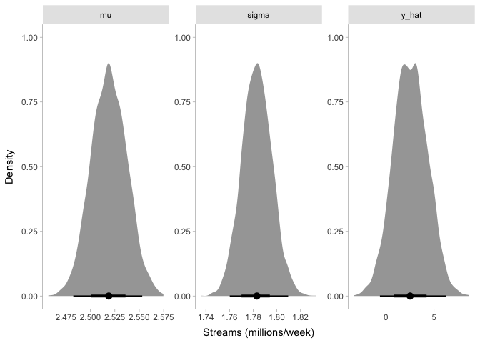
Even though our prior for mu was around one million streams per week,
it looks like our posterior is now around 2.5 million streams per week.
Likewise, the posterior for sigma is about 1.8 million, even though
our prior was centered around 0. Finally, looking at y_hat, it appears
that our model estimates the number of streams per week to be anywhere
from -500,000 to 5.5 million. Before we talk about these results any
further, though, let’s make sure that we can trust them.
Assessing model convergence
Since we don’t have direct access to the posterior distribution, Stan
uses Markov Chain Monte Carlo (MCMC) to sample values of mu and
sigma. We won’t go into the details here, but the gist is that MCMC
approximates the posterior distributions over mu and sigma by trying
to sample their values in proportion to their posterior probability. If
the samples look like they have come from the posterior distribution, we
say the model has converged. If not, we cannot use the sampled values
for inference, because they don’t reflect our posterior.
The fuzzy caterpillar check
There are few different metrics for assessing convergence of MCMC chains. Honestly, the best one is visual: the “fuzzy caterpillar” check. The idea is you plot the MCMC chains for each parameter as a function of iteration number, like so:
1
2
3
4
5
ggplot(draws, aes(x=.iteration, y=.value, color=factor(.chain))) +
    geom_line() + xlab('Iteration') + ylab('Value') +
    scale_color_discrete(name='Chain') +
    facet_grid(.variable ~ ., scales='free_y') +
    theme_tidybayes()
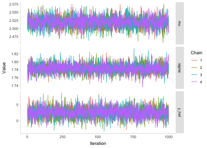
Since all of these chains look like nice fuzzy caterpillars, we can be pretty confident that they converged. To demonstrate what the chains would look like if they hadn’t converged, let’s look at the chains before the warmup period. The warmup period is the first stage of the model while it is assumed to still be converging: typically we say that something like the first half of the samples are in the warmup period, and we throw them away to be left with just the good stuff.
1
2
3
4
5
6
7
8
9
streams$draws(variables=c('mu', 'sigma', 'y_hat'),
              inc_warmup=TRUE, format='draws_df') %>%
    pivot_longer(mu:y_hat, names_to='.variable', values_to='.value') %>%
    filter(.iteration <= 250) %>%
    ggplot(aes(x=.iteration, y=.value, color=factor(.chain))) +
    geom_line() + xlab('Iteration') + ylab('Value') +
    scale_color_discrete(name='Chain') +
    facet_grid(.variable ~ ., scales='free_y') +
    theme_tidybayes()
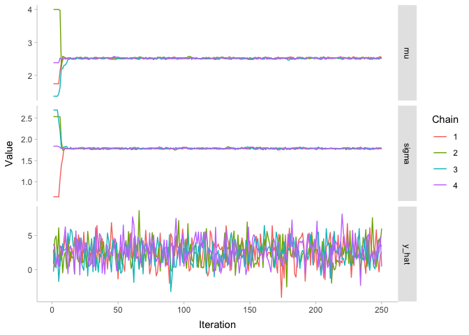
As we can see, the first 25 or so iterations do not look like nice fuzzy caterpillars. Instead, we can tell all of the four chains apart from each other, since they are close to their random initializaiton values. But by iteration 50, it appears that our model has converged: the parameters have all ended up around the values of our posterior distribution.
R-hat
If the qualitative visual check isn’t working for you, you might want something a bit more quantitative. One option is R-hat, which is the ratio of the between-chain variance and the within-chain variance of the parameter values. This gives us a good quantification of the fuzzy caterpillar check: if the between-chain variance is high (relative to the within-chain variance), the chains are all exploring different regions of the parameter space and don’t overlap much. On the other hand, if the two variances are about equal, then the chains should look like fuzzy caterpillars. Typically we look for R-hat values to be as close to 1 as possible and we start to be suspicious of poor convergence if R-hat > 1.05.
1
streams$summary() %>% select(variable, rhat)
1
2
3
4
5
6
7
## # A tibble: 4 × 2
##   variable  rhat
##   <chr>    <dbl>
## 1 lp__      1.00
## 2 mu        1.00
## 3 sigma     1.00
## 4 y_hat     1.00
Since our R-hat values are all 1.00, our model looks pretty good.
Effective Sample Size (ESS)
Related to R-hat, we can also look at the effective sample size (ESS) of
the model. Recall that we sampled 1000 draws from four MCMC chains,
resulting in 4000 total samples from the posterior. In an ideal scenario
where every iteration of the model is totally independent of the
previous iteration, this would mean that we have a sample size of 4000
samples. But most of the time, there is some amount of auto-correlation
of the parameter values between iterations. To account for this, ESS is
the sample size adjusted for within-chain auto-correlation. In other
words, even though we have 4000 samples from the posterior, because of
auto-correlation inherent in the model fitting process, we effectively
have fewer independent samples. cmdstanr actually gives us two
different ESSs: a bulk ESS and a tail ESS. The bulk ESS tells us the
effective sample size for our estimates of central tendency (i.e.,
mean/median), and the tail ESS tells us the effective sample size for
our estimates of the tail quantiles and credible intervals. Since there
are fewer samples at the tails, we will typically have a lower tail ESS
than bulk ESS. In any case, you want all of these ESSs to be as large as
possible. Minimally, it is good to have an ESS of 1000 for practical
applications.
1
streams$summary() %>% select(variable, ess_bulk, ess_tail)
1
2
3
4
5
6
7
## # A tibble: 4 × 3
##   variable ess_bulk ess_tail
##   <chr>       <dbl>    <dbl>
## 1 lp__        1862.    2564.
## 2 mu          3422.    2787.
## 3 sigma       3619.    2641.
## 4 y_hat       4012.    3890.
Our bulk ESS looks very good- all of the values are close to 4000. Though the tail ESS is lower, it is still acceptable.
Assessing model fit
Now that we know that our model converged, let’s try to figure out how well it fit. In other words, how well does our model describe the data? Just as the fuzzy-caterpillar check provides a quick & easy way of assessing convergence, posterior predictive checks do the same for model fit. To perform a posterior predictive check, all we have to do is plot the distribution of simulated data alongside the distribution of actual data:
1
2
3
4
5
6
7
8
9
10
draws %>%
    filter(.variable=='y_hat') %>%
    ggplot(aes(x=.value, fill=.variable)) +
    stat_slab(slab_alpha=.75) +
    stat_slab(slab_alpha=.75, data=tibble(.variable='y', .value=spotify2021$streams)) +
    geom_vline(xintercept=mean(spotify2021$streams)) +
    scale_fill_discrete(name='') +
    xlab('Streams (millions/week)') + ylab('Density') +
    coord_cartesian(xlim=c(-5, 10)) +
    theme_tidybayes()
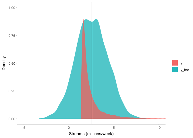
We can see that even though our model captures the mean of the stream
counts (the black vertical line) very well, there are a few problems.
First and foremost, it predicts some negative stream counts. For the top
200 songs on Spotify, not only is a negative number of streams very
unlikely, it is also impossible. Second, it predicts that most stream
counts will be at the mean, but the data have a positive skew. Let’s try
to fix these two issues at once by using a log-normal distribution
instead of a Normal distribution. The log-normal distribution is simply
what you get when you exponentiate samples from the normal distribution:
lognormal(μ,σ) = exp(Normal(μ,σ))
. So let’s try this distribution out, adjusting our priors over mu and
sigma:
1
2
3
streams_model_lognormal <- cmdstan_model('2021-12-10-streams-lognormal.stan')  ## compile the model
streams_lognormal <- streams_model_lognormal$sample(data=streams_data)
streams_lognormal
1
2
3
4
5
6
7
8
9
10
11
12
13
14
15
16
17
18
19
20
21
22
23
24
25
26
27
28
29
30
31
32
33
34
35
36
37
38
39
40
41
42
43
44
45
46
47
48
49
50
51
52
53
54
55
56
57
58
59
60
61
62
63
64
65
66
67
68
69
70
71
72
73
74
75
76
77
78
79
80
81
82
83
84
85
86
87
88
89
90
91
92
93
94
95
96
97
98
99
100
101
102
103
## Running MCMC with 4 chains, at most 20 in parallel...
##
## Chain 1 Iteration:    1 / 2000 [  0%]  (Warmup)
## Chain 1 Iteration:  100 / 2000 [  5%]  (Warmup)
## Chain 1 Iteration:  200 / 2000 [ 10%]  (Warmup)
## Chain 1 Iteration:  300 / 2000 [ 15%]  (Warmup)
## Chain 1 Iteration:  400 / 2000 [ 20%]  (Warmup)
## Chain 2 Iteration:    1 / 2000 [  0%]  (Warmup)
## Chain 2 Iteration:  100 / 2000 [  5%]  (Warmup)
## Chain 2 Iteration:  200 / 2000 [ 10%]  (Warmup)
## Chain 2 Iteration:  300 / 2000 [ 15%]  (Warmup)
## Chain 2 Iteration:  400 / 2000 [ 20%]  (Warmup)
## Chain 2 Iteration:  500 / 2000 [ 25%]  (Warmup)
## Chain 2 Iteration:  600 / 2000 [ 30%]  (Warmup)
## Chain 2 Iteration:  700 / 2000 [ 35%]  (Warmup)
## Chain 2 Iteration:  800 / 2000 [ 40%]  (Warmup)
## Chain 2 Iteration:  900 / 2000 [ 45%]  (Warmup)
## Chain 2 Iteration: 1000 / 2000 [ 50%]  (Warmup)
## Chain 2 Iteration: 1001 / 2000 [ 50%]  (Sampling)
## Chain 2 Iteration: 1100 / 2000 [ 55%]  (Sampling)
## Chain 2 Iteration: 1200 / 2000 [ 60%]  (Sampling)
## Chain 2 Iteration: 1300 / 2000 [ 65%]  (Sampling)
## Chain 2 Iteration: 1400 / 2000 [ 70%]  (Sampling)
## Chain 2 Iteration: 1500 / 2000 [ 75%]  (Sampling)
## Chain 2 Iteration: 1600 / 2000 [ 80%]  (Sampling)
## Chain 2 Iteration: 1700 / 2000 [ 85%]  (Sampling)
## Chain 2 Iteration: 1800 / 2000 [ 90%]  (Sampling)
## Chain 3 Iteration:    1 / 2000 [  0%]  (Warmup)
## Chain 3 Iteration:  100 / 2000 [  5%]  (Warmup)
## Chain 3 Iteration:  200 / 2000 [ 10%]  (Warmup)
## Chain 3 Iteration:  300 / 2000 [ 15%]  (Warmup)
## Chain 3 Iteration:  400 / 2000 [ 20%]  (Warmup)
## Chain 3 Iteration:  500 / 2000 [ 25%]  (Warmup)
## Chain 3 Iteration:  600 / 2000 [ 30%]  (Warmup)
## Chain 3 Iteration:  700 / 2000 [ 35%]  (Warmup)
## Chain 3 Iteration:  800 / 2000 [ 40%]  (Warmup)
## Chain 3 Iteration:  900 / 2000 [ 45%]  (Warmup)
## Chain 3 Iteration: 1000 / 2000 [ 50%]  (Warmup)
## Chain 3 Iteration: 1001 / 2000 [ 50%]  (Sampling)
## Chain 3 Iteration: 1100 / 2000 [ 55%]  (Sampling)
## Chain 3 Iteration: 1200 / 2000 [ 60%]  (Sampling)
## Chain 3 Iteration: 1300 / 2000 [ 65%]  (Sampling)
## Chain 3 Iteration: 1400 / 2000 [ 70%]  (Sampling)
## Chain 3 Iteration: 1500 / 2000 [ 75%]  (Sampling)
## Chain 3 Iteration: 1600 / 2000 [ 80%]  (Sampling)
## Chain 3 Iteration: 1700 / 2000 [ 85%]  (Sampling)
## Chain 3 Iteration: 1800 / 2000 [ 90%]  (Sampling)
## Chain 3 Iteration: 1900 / 2000 [ 95%]  (Sampling)
## Chain 3 Iteration: 2000 / 2000 [100%]  (Sampling)
## Chain 4 Iteration:    1 / 2000 [  0%]  (Warmup)
## Chain 4 Iteration:  100 / 2000 [  5%]  (Warmup)
## Chain 4 Iteration:  200 / 2000 [ 10%]  (Warmup)
## Chain 4 Iteration:  300 / 2000 [ 15%]  (Warmup)
## Chain 4 Iteration:  400 / 2000 [ 20%]  (Warmup)
## Chain 4 Iteration:  500 / 2000 [ 25%]  (Warmup)
## Chain 4 Iteration:  600 / 2000 [ 30%]  (Warmup)
## Chain 4 Iteration:  700 / 2000 [ 35%]  (Warmup)
## Chain 4 Iteration:  800 / 2000 [ 40%]  (Warmup)
## Chain 4 Iteration:  900 / 2000 [ 45%]  (Warmup)
## Chain 4 Iteration: 1000 / 2000 [ 50%]  (Warmup)
## Chain 4 Iteration: 1001 / 2000 [ 50%]  (Sampling)
## Chain 4 Iteration: 1100 / 2000 [ 55%]  (Sampling)
## Chain 4 Iteration: 1200 / 2000 [ 60%]  (Sampling)
## Chain 4 Iteration: 1300 / 2000 [ 65%]  (Sampling)
## Chain 4 Iteration: 1400 / 2000 [ 70%]  (Sampling)
## Chain 4 Iteration: 1500 / 2000 [ 75%]  (Sampling)
## Chain 4 Iteration: 1600 / 2000 [ 80%]  (Sampling)
## Chain 4 Iteration: 1700 / 2000 [ 85%]  (Sampling)
## Chain 4 Iteration: 1800 / 2000 [ 90%]  (Sampling)
## Chain 4 Iteration: 1900 / 2000 [ 95%]  (Sampling)
## Chain 4 Iteration: 2000 / 2000 [100%]  (Sampling)
## Chain 1 Iteration:  500 / 2000 [ 25%]  (Warmup)
## Chain 1 Iteration:  600 / 2000 [ 30%]  (Warmup)
## Chain 1 Iteration:  700 / 2000 [ 35%]  (Warmup)
## Chain 1 Iteration:  800 / 2000 [ 40%]  (Warmup)
## Chain 1 Iteration:  900 / 2000 [ 45%]  (Warmup)
## Chain 1 Iteration: 1000 / 2000 [ 50%]  (Warmup)
## Chain 1 Iteration: 1001 / 2000 [ 50%]  (Sampling)
## Chain 1 Iteration: 1100 / 2000 [ 55%]  (Sampling)
## Chain 1 Iteration: 1200 / 2000 [ 60%]  (Sampling)
## Chain 1 Iteration: 1300 / 2000 [ 65%]  (Sampling)
## Chain 1 Iteration: 1400 / 2000 [ 70%]  (Sampling)
## Chain 1 Iteration: 1500 / 2000 [ 75%]  (Sampling)
## Chain 1 Iteration: 1600 / 2000 [ 80%]  (Sampling)
## Chain 1 Iteration: 1700 / 2000 [ 85%]  (Sampling)
## Chain 1 Iteration: 1800 / 2000 [ 90%]  (Sampling)
## Chain 1 Iteration: 1900 / 2000 [ 95%]  (Sampling)
## Chain 1 Iteration: 2000 / 2000 [100%]  (Sampling)
## Chain 1 finished in 0.5 seconds.
## Chain 2 Iteration: 1900 / 2000 [ 95%]  (Sampling)
## Chain 2 Iteration: 2000 / 2000 [100%]  (Sampling)
## Chain 2 finished in 0.5 seconds.
## Chain 3 finished in 0.6 seconds.
## Chain 4 finished in 0.6 seconds.
##
## All 4 chains finished successfully.
## Mean chain execution time: 0.5 seconds.
## Total execution time: 1.1 seconds.
##  variable     mean   median   sd  mad       q5      q95 rhat ess_bulk ess_tail
##     lp__  -5789.20 -5788.89 0.97 0.67 -5791.16 -5788.29 1.00     1990     2763
##     mu        0.81     0.81 0.00 0.00     0.81     0.82 1.00     4259     3110
##     sigma     0.45     0.45 0.00 0.00     0.44     0.45 1.00     3122     2651
##     y_hat     2.51     2.28 1.20 0.97     1.08     4.77 1.00     3558     3888
1
2
3
4
5
6
7
8
9
10
11
streams_lognormal %>%
    gather_draws(y_hat) %>%
    ggplot(aes(x=.value, fill=.variable)) +
    stat_slab(slab_alpha=.75, fill=NA, color='black', data=filter(draws, .variable=='y_hat') %>% mutate(.variable='y_hat (normal)')) +
    stat_slab(slab_alpha=.75) +
    stat_slab(slab_alpha=.75, data=tibble(.variable='y', .value=spotify2021$streams)) +
    geom_vline(xintercept=mean(spotify2021$streams)) +
    scale_fill_discrete(name='') +
    xlab('Streams (millions/week)') + ylab('Density') +
    coord_cartesian(xlim=c(-5, 10)) +
    theme_tidybayes()
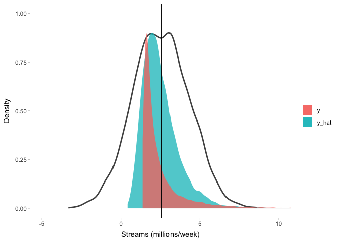
Clearly this model (blue) does a lot better at describing stream counts than the previous one (black line), but it’s not perfect either. Importantly, there is no single gold standard for model fit: a model that fits perfectly fine for some purposes may not be good for other purposes. So it is up to you, the modeler, to determine when your model is good enough to inspect.
Linear Regression in Stan
Modeling the mean and standard deviation of just one datapoint is good and well, but as scientists we’re usually more interested in effects. To do that, we’re going to need to add some predictor variables to our model. To switch things up, let’s say we want to predict the energy level of a song given the song’s loudness. First, let’s take a look at the data:
1
2
3
ggplot(spotify2021, aes(x=loudness, y=energy)) +
    geom_point(alpha=.2) +
    theme_tidybayes()
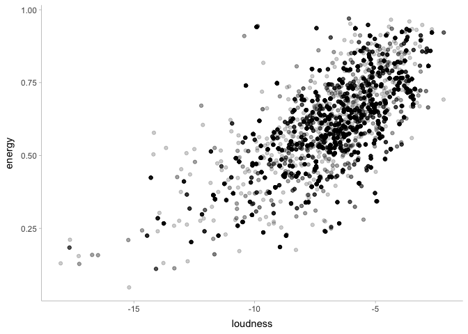
This certainly looks promising! Let’s write a Stan program to see if this is the case:
1
2
3
4
5
6
7
8
9
10
11
12
13
14
15
16
17
18
19
20
21
22
23
24
25
26
27
data {
  int<lower=0> N;                 // the number of data points
  vector[N] x;                    // the loudness of each song
  vector<lower=0, upper=1>[N] y;  // the energy level of each song
}

parameters {
  real alpha;
  real beta;
  real<lower=0> sigma;
}

transformed parameters {
  vector[N] mu = alpha + beta*x;
}

model {
  alpha ~ normal(.5, .5);
  beta ~ normal(0, .1);
  sigma ~ normal(0, 1);

  y ~ normal(mu, sigma);
}

generated quantities {
  real y_hat[N] = normal_rng(mu, sigma);
}
Hopefully by now most of this new model looks familiar: we’re modeling
energy as normally distributed with mean mu and standard deviation
sigma. However, now instead of estimating a single mu, we’re
calculating mu as a transformed parameter based on three things.
Unsurprisingly, x is the vector of loudness values for each track.
alpha is the intercept, which represents the mean energy level when
loudness == 0. And finally, beta is the slope, which represents the
average change in energy for every decible increase in loudness. The
reason we declare mu as a transformed parameter instead of a regular
old parameter is that it makes sampling more efficient: by doing so,
we’re telling Stan that mu is just some combination of the other
parameters, so we don’t need to sample it directly (we can just sample
alpha and beta). I’ve assigned normal priors for each parameter based on
sheer intuition: hopefully none of the results should vary if these are
set slightly differently.
The last thing to note is that now we’re estimating a unique y_hat for
each individual data point. The reasoning behind this is that each data
point now has a unique prediction of energy (before, the estimates did
not depend on predictors).
1
2
3
4
energy_data <- list(N=nrow(spotify2021), x=spotify2021$loudness, y=spotify2021$energy)
energy_model <- cmdstan_model('2021-12-10-energy.stan')  ## compile the model
energy <- energy_model$sample(data=energy_data)
energy
1
2
3
4
5
6
7
8
9
10
11
12
13
14
15
16
17
18
19
20
21
22
23
24
25
26
27
28
29
30
31
32
33
34
35
36
37
38
39
40
41
42
43
44
45
46
47
48
49
50
51
52
53
54
55
56
57
58
59
60
61
62
63
64
65
66
67
68
69
70
71
72
73
74
75
76
77
78
79
80
81
82
83
84
85
86
87
88
89
90
91
92
93
94
95
96
97
98
99
100
101
102
103
104
105
106
107
108
109
110
111
## Running MCMC with 4 chains, at most 20 in parallel...
##
## Chain 1 Iteration:    1 / 2000 [  0%]  (Warmup)
## Chain 2 Iteration:    1 / 2000 [  0%]  (Warmup)
## Chain 2 Iteration:  100 / 2000 [  5%]  (Warmup)
## Chain 3 Iteration:    1 / 2000 [  0%]  (Warmup)
## Chain 3 Iteration:  100 / 2000 [  5%]  (Warmup)
## Chain 4 Iteration:    1 / 2000 [  0%]  (Warmup)
## Chain 4 Iteration:  100 / 2000 [  5%]  (Warmup)
## Chain 1 Iteration:  100 / 2000 [  5%]  (Warmup)
## Chain 3 Iteration:  200 / 2000 [ 10%]  (Warmup)
## Chain 4 Iteration:  200 / 2000 [ 10%]  (Warmup)
## Chain 2 Iteration:  200 / 2000 [ 10%]  (Warmup)
## Chain 3 Iteration:  300 / 2000 [ 15%]  (Warmup)
## Chain 1 Iteration:  200 / 2000 [ 10%]  (Warmup)
## Chain 3 Iteration:  400 / 2000 [ 20%]  (Warmup)
## Chain 4 Iteration:  300 / 2000 [ 15%]  (Warmup)
## Chain 2 Iteration:  300 / 2000 [ 15%]  (Warmup)
## Chain 4 Iteration:  400 / 2000 [ 20%]  (Warmup)
## Chain 1 Iteration:  300 / 2000 [ 15%]  (Warmup)
## Chain 3 Iteration:  500 / 2000 [ 25%]  (Warmup)
## Chain 2 Iteration:  400 / 2000 [ 20%]  (Warmup)
## Chain 3 Iteration:  600 / 2000 [ 30%]  (Warmup)
## Chain 1 Iteration:  400 / 2000 [ 20%]  (Warmup)
## Chain 4 Iteration:  500 / 2000 [ 25%]  (Warmup)
## Chain 2 Iteration:  500 / 2000 [ 25%]  (Warmup)
## Chain 3 Iteration:  700 / 2000 [ 35%]  (Warmup)
## Chain 1 Iteration:  500 / 2000 [ 25%]  (Warmup)
## Chain 4 Iteration:  600 / 2000 [ 30%]  (Warmup)
## Chain 2 Iteration:  600 / 2000 [ 30%]  (Warmup)
## Chain 3 Iteration:  800 / 2000 [ 40%]  (Warmup)
## Chain 4 Iteration:  700 / 2000 [ 35%]  (Warmup)
## Chain 1 Iteration:  600 / 2000 [ 30%]  (Warmup)
## Chain 2 Iteration:  700 / 2000 [ 35%]  (Warmup)
## Chain 3 Iteration:  900 / 2000 [ 45%]  (Warmup)
## Chain 4 Iteration:  800 / 2000 [ 40%]  (Warmup)
## Chain 1 Iteration:  700 / 2000 [ 35%]  (Warmup)
## Chain 2 Iteration:  800 / 2000 [ 40%]  (Warmup)
## Chain 3 Iteration: 1000 / 2000 [ 50%]  (Warmup)
## Chain 3 Iteration: 1001 / 2000 [ 50%]  (Sampling)
## Chain 4 Iteration:  900 / 2000 [ 45%]  (Warmup)
## Chain 1 Iteration:  800 / 2000 [ 40%]  (Warmup)
## Chain 2 Iteration:  900 / 2000 [ 45%]  (Warmup)
## Chain 4 Iteration: 1000 / 2000 [ 50%]  (Warmup)
## Chain 4 Iteration: 1001 / 2000 [ 50%]  (Sampling)
## Chain 1 Iteration:  900 / 2000 [ 45%]  (Warmup)
## Chain 2 Iteration: 1000 / 2000 [ 50%]  (Warmup)
## Chain 2 Iteration: 1001 / 2000 [ 50%]  (Sampling)
## Chain 3 Iteration: 1100 / 2000 [ 55%]  (Sampling)
## Chain 1 Iteration: 1000 / 2000 [ 50%]  (Warmup)
## Chain 1 Iteration: 1001 / 2000 [ 50%]  (Sampling)
## Chain 4 Iteration: 1100 / 2000 [ 55%]  (Sampling)
## Chain 2 Iteration: 1100 / 2000 [ 55%]  (Sampling)
## Chain 3 Iteration: 1200 / 2000 [ 60%]  (Sampling)
## Chain 1 Iteration: 1100 / 2000 [ 55%]  (Sampling)
## Chain 4 Iteration: 1200 / 2000 [ 60%]  (Sampling)
## Chain 2 Iteration: 1200 / 2000 [ 60%]  (Sampling)
## Chain 3 Iteration: 1300 / 2000 [ 65%]  (Sampling)
## Chain 1 Iteration: 1200 / 2000 [ 60%]  (Sampling)
## Chain 4 Iteration: 1300 / 2000 [ 65%]  (Sampling)
## Chain 2 Iteration: 1300 / 2000 [ 65%]  (Sampling)
## Chain 3 Iteration: 1400 / 2000 [ 70%]  (Sampling)
## Chain 1 Iteration: 1300 / 2000 [ 65%]  (Sampling)
## Chain 2 Iteration: 1400 / 2000 [ 70%]  (Sampling)
## Chain 4 Iteration: 1400 / 2000 [ 70%]  (Sampling)
## Chain 3 Iteration: 1500 / 2000 [ 75%]  (Sampling)
## Chain 4 Iteration: 1500 / 2000 [ 75%]  (Sampling)
## Chain 1 Iteration: 1400 / 2000 [ 70%]  (Sampling)
## Chain 2 Iteration: 1500 / 2000 [ 75%]  (Sampling)
## Chain 3 Iteration: 1600 / 2000 [ 80%]  (Sampling)
## Chain 4 Iteration: 1600 / 2000 [ 80%]  (Sampling)
## Chain 1 Iteration: 1500 / 2000 [ 75%]  (Sampling)
## Chain 2 Iteration: 1600 / 2000 [ 80%]  (Sampling)
## Chain 3 Iteration: 1700 / 2000 [ 85%]  (Sampling)
## Chain 1 Iteration: 1600 / 2000 [ 80%]  (Sampling)
## Chain 4 Iteration: 1700 / 2000 [ 85%]  (Sampling)
## Chain 2 Iteration: 1700 / 2000 [ 85%]  (Sampling)
## Chain 3 Iteration: 1800 / 2000 [ 90%]  (Sampling)
## Chain 4 Iteration: 1800 / 2000 [ 90%]  (Sampling)
## Chain 2 Iteration: 1800 / 2000 [ 90%]  (Sampling)
## Chain 3 Iteration: 1900 / 2000 [ 95%]  (Sampling)
## Chain 1 Iteration: 1700 / 2000 [ 85%]  (Sampling)
## Chain 4 Iteration: 1900 / 2000 [ 95%]  (Sampling)
## Chain 2 Iteration: 1900 / 2000 [ 95%]  (Sampling)
## Chain 3 Iteration: 2000 / 2000 [100%]  (Sampling)
## Chain 3 finished in 16.5 seconds.
## Chain 1 Iteration: 1800 / 2000 [ 90%]  (Sampling)
## Chain 4 Iteration: 2000 / 2000 [100%]  (Sampling)
## Chain 4 finished in 17.5 seconds.
## Chain 2 Iteration: 2000 / 2000 [100%]  (Sampling)
## Chain 2 finished in 17.7 seconds.
## Chain 1 Iteration: 1900 / 2000 [ 95%]  (Sampling)
## Chain 1 Iteration: 2000 / 2000 [100%]  (Sampling)
## Chain 1 finished in 19.0 seconds.
##
## All 4 chains finished successfully.
## Mean chain execution time: 17.7 seconds.
## Total execution time: 19.1 seconds.
##  variable     mean   median   sd  mad       q5      q95 rhat ess_bulk ess_tail
##     lp__  15649.15 15649.50 1.20 1.04 15646.70 15650.50 1.00     1272     1456
##     alpha     0.94     0.94 0.00 0.00     0.93     0.95 1.00     1541     1279
##     beta      0.05     0.05 0.00 0.00     0.05     0.05 1.00     1615     1370
##     sigma     0.11     0.11 0.00 0.00     0.11     0.12 1.00     1672     1556
##     mu[1]     0.53     0.53 0.00 0.00     0.53     0.53 1.00     3470     2550
##     mu[2]     0.55     0.55 0.00 0.00     0.54     0.55 1.00     3798     2745
##     mu[3]     0.62     0.62 0.00 0.00     0.62     0.62 1.00     3817     2854
##     mu[4]     0.77     0.77 0.00 0.00     0.76     0.77 1.00     1671     1721
##     mu[5]     0.64     0.64 0.00 0.00     0.64     0.64 1.00     3293     2835
##     mu[6]     0.45     0.45 0.00 0.00     0.44     0.45 1.00     2417     2182
##
##  # showing 10 of 18804 rows (change via 'max_rows' argument or 'cmdstanr_max_rows' option)
The results show that there does appear to be a sizable increase in energy with loudness! Let’s plot the coefficients to make this more clear:
1
2
3
4
5
6
7
energy %>%
    gather_draws(alpha, beta, sigma) %>%
    ggplot(aes(x=.value)) +
    stat_halfeye(point_interval=median_hdi, normalize='panels') +
    xlab('Value') + ylab('Parameter') +
    facet_wrap(~ .variable, scales='free') +
    theme_tidybayes()
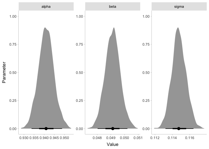
Since the coefficient beta is clearly greater than zero, we can say we
found an effect! If you’re skeptical, it might help to know that the
frequentist parameter values are extremely similar:
1
summary(lm(energy ~ loudness, spotify2021))
1
2
3
4
5
6
7
8
9
10
11
12
13
14
15
16
17
18
##
## Call:
## lm(formula = energy ~ loudness, data = spotify2021)
##
## Residuals:
##      Min       1Q   Median       3Q      Max
## -0.39105 -0.06769 -0.00484  0.07276  0.48819
##
## Coefficients:
##              Estimate Std. Error t value Pr(>|t|)
## (Intercept) 0.9410411  0.0038950  241.60   <2e-16 ***
## loudness    0.0491423  0.0005569   88.23   <2e-16 ***
## ---
## Signif. codes:  0 '***' 0.001 '**' 0.01 '*' 0.05 '.' 0.1 ' ' 1
##
## Residual standard error: 0.1147 on 9398 degrees of freedom
## Multiple R-squared:  0.4531, Adjusted R-squared:  0.453
## F-statistic:  7785 on 1 and 9398 DF,  p-value: < 2.2e-16
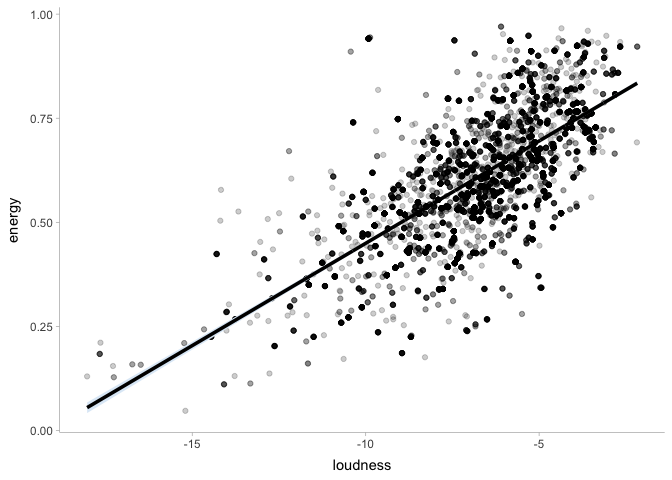
Let’s plot our regression line on top of the data:
1
2
3
4
5
6
7
8
9
10
energy_draws <- energy %>%
    spread_draws(mu[.row]) %>%
    mutate(x=spotify2021$loudness[.row])

ggplot(spotify2021, aes(x=loudness, y=energy)) +
    geom_point(alpha=.2) +
    stat_lineribbon(aes(x=x, y=mu), data=energy_draws,
                    .width=.95, show.legend=FALSE) +
    scale_fill_brewer() +
    theme_tidybayes()
If needed, we can also use the posterior distribution to compute other
quantities of interest. For example, let’s calculate the coefficient of
variation, R^2:
1
2
3
4
5
6
7
8
9
10
11
12
energy_R2 <- energy %>%
    spread_draws(mu[.row]) %>%
    left_join(tibble(.row=1:nrow(spotify2021), y=spotify2021$energy)) %>%
    group_by(.draw) %>%
    summarize(ss_total=sum((y-mean(y))^2),
              ss_residual=sum((y-mu)^2),
              R2=1 - ss_residual/ss_total)

ggplot(energy_R2, aes(x=R2)) +
    stat_halfeye(point_interval=median_hdi) +
    xlab('R^2') + ylab('Density') +
    theme_tidybayes()
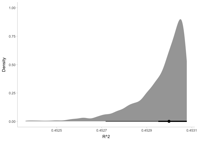
This plot shows us that our model is pretty darn good: it explains about 45% of the variance in energy!
Entering the matrix
To round off this tutorial, let’s try to make our regression model a little more general. Right now, we only have one predictor variable coded into our model. What if we wanted to allow for more than one variable and interactions between variables? As we talked about in Pranjal’s fantastic tutorial on linear algebra, the way to achieve this is to use matrices. This might sound scary, but really the core idea is still the same.
Let’s go back to stream counts: presume that we want to know what makes the top 200 songs so successful. Is it their energy, their danceability, duration, or some combination of variables? To find out, let’s code a Stan model. To keep things simple, I’m going to ignore the skew in the data and fit a model with a normal likelihood.
1
2
3
4
5
6
7
8
9
10
11
12
13
14
15
16
17
18
19
20
21
22
23
24
25
26
27
28
data {
  int<lower=0> N;      // the number of data points
  int<lower=0> K;      // the number of regression coefficients
  matrix[N, K] X;      // the predictor variables
  vector[N] y;         // the outcome variable
}

parameters {
  real alpha;
  vector[K] beta;
  real<lower=0> sigma;
}

transformed parameters {
  vector[N] mu = alpha + X*beta;
}

model {
  alpha ~ normal(0, 1);
  beta ~ normal(0, 1);
  sigma ~ normal(0, 1);

  y ~ normal(mu, sigma);
}

generated quantities {
  real y_hat[N] = normal_rng(mu, sigma);
}
As promised, there are only a few differences between this model and the
last. The most obvious difference is that while x used to be an
N-vector with one value for each data point, X is now an N by K
matrix with one row of K predictors for each data point. To make this
clear, I changed from little x to big X in the code. The other main
difference is that before we used to have a single scalar beta, which
represented the effect of x on y. But now that we have K different
x’s, beta is now a K-vector, where each element represents the
effect of the Kth predictor variable on y. What’s nice about Stan is
that everything else works just as before! Stan recognizes that beta*X
is now a vector-matrix multiplication, and it can perform the whole
multiplication out with the same code. If you think it’s more clear, you
always have the option of writing out some loops for this
multiplication:
1
2
3
4
5
6
7
8
9
10
11
12
13
transformed parameters {
  vector[N] mu;

  // loop over data points
  for (i in 1:N) {
    mu[i] = alpha;

    // loop over predictor variables
    for (k in 1:K) {
      mu[i] = mu[i] + beta[k]*X[n,k];
    }
  }
}
While the other version of the code was a single line, this version is 7 lines of code! And the worse part is that even though this code is longer, it’s actually slower to execute, since Stan can internally optimize matrix multiplication but it can’t internally optimize these sorts of loops. So unless you need to expand out the multiplication, it’s generally better to use the shorter version.
Now that we have our model, let’s try to predict stream counts using duration and tempo:
1
2
3
4
5
6
streams_data <- list(N=nrow(spotify2021), K=2,
                     X=select(spotify2021, duration_ms, tempo),
                     y=spotify2021$streams)
streams_model <- cmdstan_model('2021-12-10-streams-glm.stan')  ## compile the model
streams <- streams_model$sample(data=streams_data)
streams
1
2
3
4
5
6
7
8
9
10
11
12
13
14
15
16
17
18
19
20
21
22
23
24
25
26
27
28
29
30
31
32
33
34
35
36
37
38
39
40
41
42
43
44
45
46
47
48
49
50
51
52
53
54
55
56
57
58
59
60
61
62
63
64
65
66
67
68
69
70
71
72
73
74
75
76
77
78
79
80
81
82
83
84
85
86
87
88
89
90
91
92
93
94
95
96
97
98
99
100
101
102
103
104
105
106
107
108
109
110
111
112
113
114
115
116
117
118
119
120
121
122
## Running MCMC with 4 chains, at most 20 in parallel...
##
## Chain 1 Iteration:    1 / 2000 [  0%]  (Warmup)
## Chain 1 Iteration:  100 / 2000 [  5%]  (Warmup)
## Chain 2 Iteration:    1 / 2000 [  0%]  (Warmup)
## Chain 3 Iteration:    1 / 2000 [  0%]  (Warmup)
## Chain 4 Iteration:    1 / 2000 [  0%]  (Warmup)
## Chain 1 Iteration:  200 / 2000 [ 10%]  (Warmup)
## Chain 1 Iteration:  300 / 2000 [ 15%]  (Warmup)
## Chain 1 Iteration:  400 / 2000 [ 20%]  (Warmup)
## Chain 1 Iteration:  500 / 2000 [ 25%]  (Warmup)
## Chain 3 Iteration:  100 / 2000 [  5%]  (Warmup)
## Chain 1 Iteration:  600 / 2000 [ 30%]  (Warmup)
## Chain 1 Iteration:  700 / 2000 [ 35%]  (Warmup)
## Chain 1 Iteration:  800 / 2000 [ 40%]  (Warmup)
## Chain 1 Iteration:  900 / 2000 [ 45%]  (Warmup)
## Chain 1 Iteration: 1000 / 2000 [ 50%]  (Warmup)
## Chain 1 Iteration: 1001 / 2000 [ 50%]  (Sampling)
## Chain 3 Iteration:  200 / 2000 [ 10%]  (Warmup)
## Chain 2 Iteration:  100 / 2000 [  5%]  (Warmup)
## Chain 1 Iteration: 1100 / 2000 [ 55%]  (Sampling)
## Chain 3 Iteration:  300 / 2000 [ 15%]  (Warmup)
## Chain 1 Iteration: 1200 / 2000 [ 60%]  (Sampling)
## Chain 3 Iteration:  400 / 2000 [ 20%]  (Warmup)
## Chain 1 Iteration: 1300 / 2000 [ 65%]  (Sampling)
## Chain 1 Iteration: 1400 / 2000 [ 70%]  (Sampling)
## Chain 3 Iteration:  500 / 2000 [ 25%]  (Warmup)
## Chain 1 Iteration: 1500 / 2000 [ 75%]  (Sampling)
## Chain 3 Iteration:  600 / 2000 [ 30%]  (Warmup)
## Chain 1 Iteration: 1600 / 2000 [ 80%]  (Sampling)
## Chain 4 Iteration:  100 / 2000 [  5%]  (Warmup)
## Chain 3 Iteration:  700 / 2000 [ 35%]  (Warmup)
## Chain 1 Iteration: 1700 / 2000 [ 85%]  (Sampling)
## Chain 1 Iteration: 1800 / 2000 [ 90%]  (Sampling)
## Chain 3 Iteration:  800 / 2000 [ 40%]  (Warmup)
## Chain 2 Iteration:  200 / 2000 [ 10%]  (Warmup)
## Chain 1 Iteration: 1900 / 2000 [ 95%]  (Sampling)
## Chain 3 Iteration:  900 / 2000 [ 45%]  (Warmup)
## Chain 1 Iteration: 2000 / 2000 [100%]  (Sampling)
## Chain 1 finished in 10.3 seconds.
## Chain 3 Iteration: 1000 / 2000 [ 50%]  (Warmup)
## Chain 3 Iteration: 1001 / 2000 [ 50%]  (Sampling)
## Chain 3 Iteration: 1100 / 2000 [ 55%]  (Sampling)
## Chain 3 Iteration: 1200 / 2000 [ 60%]  (Sampling)
## Chain 2 Iteration:  300 / 2000 [ 15%]  (Warmup)
## Chain 3 Iteration: 1300 / 2000 [ 65%]  (Sampling)
## Chain 3 Iteration: 1400 / 2000 [ 70%]  (Sampling)
## Chain 3 Iteration: 1500 / 2000 [ 75%]  (Sampling)
## Chain 2 Iteration:  400 / 2000 [ 20%]  (Warmup)
## Chain 4 Iteration:  200 / 2000 [ 10%]  (Warmup)
## Chain 3 Iteration: 1600 / 2000 [ 80%]  (Sampling)
## Chain 3 Iteration: 1700 / 2000 [ 85%]  (Sampling)
## Chain 3 Iteration: 1800 / 2000 [ 90%]  (Sampling)
## Chain 3 Iteration: 1900 / 2000 [ 95%]  (Sampling)
## Chain 3 Iteration: 2000 / 2000 [100%]  (Sampling)
## Chain 3 finished in 24.6 seconds.
## Chain 4 Iteration:  300 / 2000 [ 15%]  (Warmup)
## Chain 2 Iteration:  500 / 2000 [ 25%]  (Warmup)
## Chain 4 Iteration:  400 / 2000 [ 20%]  (Warmup)
## Chain 4 Iteration:  500 / 2000 [ 25%]  (Warmup)
## Chain 4 Iteration:  600 / 2000 [ 30%]  (Warmup)
## Chain 2 Iteration:  600 / 2000 [ 30%]  (Warmup)
## Chain 4 Iteration:  700 / 2000 [ 35%]  (Warmup)
## Chain 4 Iteration:  800 / 2000 [ 40%]  (Warmup)
## Chain 2 Iteration:  700 / 2000 [ 35%]  (Warmup)
## Chain 4 Iteration:  900 / 2000 [ 45%]  (Warmup)
## Chain 2 Iteration:  800 / 2000 [ 40%]  (Warmup)
## Chain 4 Iteration: 1000 / 2000 [ 50%]  (Warmup)
## Chain 4 Iteration: 1001 / 2000 [ 50%]  (Sampling)
## Chain 2 Iteration:  900 / 2000 [ 45%]  (Warmup)
## Chain 4 Iteration: 1100 / 2000 [ 55%]  (Sampling)
## Chain 2 Iteration: 1000 / 2000 [ 50%]  (Warmup)
## Chain 2 Iteration: 1001 / 2000 [ 50%]  (Sampling)
## Chain 2 Iteration: 1100 / 2000 [ 55%]  (Sampling)
## Chain 2 Iteration: 1200 / 2000 [ 60%]  (Sampling)
## Chain 4 Iteration: 1200 / 2000 [ 60%]  (Sampling)
## Chain 2 Iteration: 1300 / 2000 [ 65%]  (Sampling)
## Chain 2 Iteration: 1400 / 2000 [ 70%]  (Sampling)
## Chain 2 Iteration: 1500 / 2000 [ 75%]  (Sampling)
## Chain 2 Iteration: 1600 / 2000 [ 80%]  (Sampling)
## Chain 2 Iteration: 1700 / 2000 [ 85%]  (Sampling)
## Chain 2 Iteration: 1800 / 2000 [ 90%]  (Sampling)
## Chain 2 Iteration: 1900 / 2000 [ 95%]  (Sampling)
## Chain 2 Iteration: 2000 / 2000 [100%]  (Sampling)
## Chain 2 finished in 119.5 seconds.
## Chain 4 Iteration: 1300 / 2000 [ 65%]  (Sampling)
## Chain 4 Iteration: 1400 / 2000 [ 70%]  (Sampling)
## Chain 4 Iteration: 1500 / 2000 [ 75%]  (Sampling)
## Chain 4 Iteration: 1600 / 2000 [ 80%]  (Sampling)
## Chain 4 Iteration: 1700 / 2000 [ 85%]  (Sampling)
## Chain 4 Iteration: 1800 / 2000 [ 90%]  (Sampling)
## Chain 4 Iteration: 1900 / 2000 [ 95%]  (Sampling)
## Chain 4 Iteration: 2000 / 2000 [100%]  (Sampling)
## Chain 4 finished in 247.5 seconds.
##
## All 4 chains finished successfully.
## Mean chain execution time: 100.5 seconds.
## Total execution time: 247.6 seconds.
##  variable        mean     median         sd       mad           q5       q95
##   lp__    -5158838.53 -152326.00 8680417.44 210440.84 -20199705.00 -10386.00
##   alpha          0.36       0.48       1.21      1.19        -1.45      1.93
##   beta[1]        0.00       0.00       0.00      0.00         0.00      0.00
##   beta[2]        0.20       0.01       0.51      0.17        -0.28      1.06
##   sigma          1.79       1.50       1.09      0.91         0.65      3.32
##   mu[1]         -5.03       2.84      20.73      7.29       -40.00     14.76
##   mu[2]          3.39       2.46       2.45      0.98         1.01      7.51
##   mu[3]          4.02       2.35       4.42      1.72        -0.27     11.45
##   mu[4]          3.73       2.13       4.42      1.91        -0.66     11.14
##   mu[5]          7.77       2.66      13.40      4.58        -4.93     30.41
##  rhat ess_bulk ess_tail
##  3.57        4       11
##  3.55        4        8
##  4.08        4       10
##  4.23        4       11
##  4.29        4       11
##  4.05        4       10
##  3.59        4       10
##  3.87        4       10
##  3.96        4       10
##  3.36        4       10
##
##  # showing 10 of 18805 rows (change via 'max_rows' argument or 'cmdstanr_max_rows' option)
Oh, that doesn’t look good… what went wrong? In addition to taking really long to fit, we get some scary warnings, and the R-hat values are huge! Let’s look at the chains:
1
2
3
4
5
6
7
streams$draws(c('alpha', 'beta', 'sigma'), format='draws_df') %>%
    pivot_longer(alpha:sigma, names_to='.variable', values_to='.value') %>%
    ggplot(aes(x=.iteration, y=.value, color=factor(.chain))) +
    geom_line() + xlab('Iteration') + ylab('Value') +
    scale_color_discrete(name='Chain') +
    facet_grid(.variable ~ ., scales='free_y') +
    theme_tidybayes()
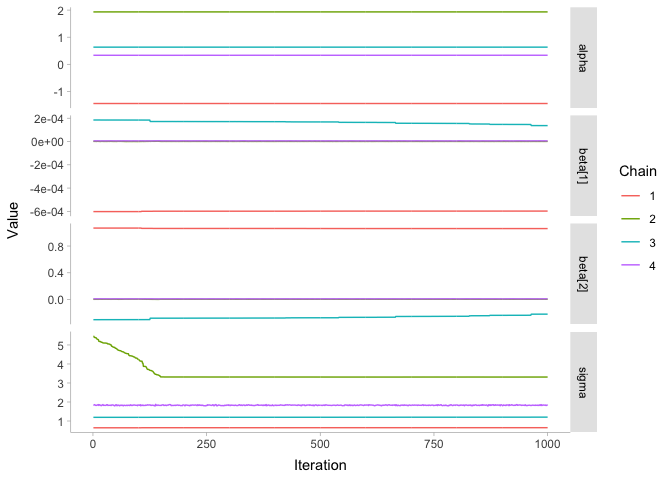
These are some bad looking chains! To get an idea of what went wrong, let’s take another quick look at our data:
1
summary(streams_data$X)
1
2
3
4
5
6
7
##   duration_ms         tempo
##  Min.   : 52062   Min.   : 40.32
##  1st Qu.:167916   1st Qu.: 97.69
##  Median :195873   Median :121.97
##  Mean   :198911   Mean   :121.97
##  3rd Qu.:221980   3rd Qu.:142.59
##  Max.   :690732   Max.   :208.92
One thing stands out to me: the scale of duration_ms is much much
larger than that of tempo and loudness. This can actually cause
problems in prior specification and model fitting, because Stan doesn’t
know that since duration_ms is much larger, its beta weights should
be very small, whereas the other beta weights will probably be larger.
Although we could z-score all of our variables to have the same scale
for all of our betas, it would be nice to retain the scales of the
variables, since they are meaningful (e.g., beats per minute is more
inherently meaningful than standard deviations of beats per minute). So,
let’s try our model again, but using duration in seconds rather than
milliseconds:
1
2
3
4
5
6
7
spotify2021$duration_s <- spotify2021$duration_ms / 1000

streams_data <- list(N=nrow(spotify2021), K=2,
                     X=select(spotify2021, duration_s, tempo),
                     y=spotify2021$streams)
streams <- streams_model$sample(data=streams_data)
streams
1
2
3
4
5
6
7
8
9
10
11
12
13
14
15
16
17
18
19
20
21
22
23
24
25
26
27
28
29
30
31
32
33
34
35
36
37
38
39
40
41
42
43
44
45
46
47
48
49
50
51
52
53
54
55
56
57
58
59
60
61
62
63
64
65
66
67
68
69
70
71
72
73
74
75
76
77
78
79
80
81
82
83
84
85
86
87
88
89
90
91
92
93
94
95
96
97
98
99
100
101
102
103
104
105
106
107
108
109
110
111
112
113
114
115
116
117
118
119
120
121
122
## Running MCMC with 4 chains, at most 20 in parallel...
##
## Chain 1 Iteration:    1 / 2000 [  0%]  (Warmup)
## Chain 2 Iteration:    1 / 2000 [  0%]  (Warmup)
## Chain 3 Iteration:    1 / 2000 [  0%]  (Warmup)
## Chain 4 Iteration:    1 / 2000 [  0%]  (Warmup)
## Chain 2 Iteration:  100 / 2000 [  5%]  (Warmup)
## Chain 3 Iteration:  100 / 2000 [  5%]  (Warmup)
## Chain 3 Iteration:  200 / 2000 [ 10%]  (Warmup)
## Chain 2 Iteration:  200 / 2000 [ 10%]  (Warmup)
## Chain 3 Iteration:  300 / 2000 [ 15%]  (Warmup)
## Chain 1 Iteration:  100 / 2000 [  5%]  (Warmup)
## Chain 4 Iteration:  100 / 2000 [  5%]  (Warmup)
## Chain 3 Iteration:  400 / 2000 [ 20%]  (Warmup)
## Chain 2 Iteration:  300 / 2000 [ 15%]  (Warmup)
## Chain 3 Iteration:  500 / 2000 [ 25%]  (Warmup)
## Chain 2 Iteration:  400 / 2000 [ 20%]  (Warmup)
## Chain 3 Iteration:  600 / 2000 [ 30%]  (Warmup)
## Chain 1 Iteration:  200 / 2000 [ 10%]  (Warmup)
## Chain 3 Iteration:  700 / 2000 [ 35%]  (Warmup)
## Chain 3 Iteration:  800 / 2000 [ 40%]  (Warmup)
## Chain 2 Iteration:  500 / 2000 [ 25%]  (Warmup)
## Chain 3 Iteration:  900 / 2000 [ 45%]  (Warmup)
## Chain 1 Iteration:  300 / 2000 [ 15%]  (Warmup)
## Chain 4 Iteration:  200 / 2000 [ 10%]  (Warmup)
## Chain 2 Iteration:  600 / 2000 [ 30%]  (Warmup)
## Chain 3 Iteration: 1000 / 2000 [ 50%]  (Warmup)
## Chain 3 Iteration: 1001 / 2000 [ 50%]  (Sampling)
## Chain 1 Iteration:  400 / 2000 [ 20%]  (Warmup)
## Chain 2 Iteration:  700 / 2000 [ 35%]  (Warmup)
## Chain 3 Iteration: 1100 / 2000 [ 55%]  (Sampling)
## Chain 4 Iteration:  300 / 2000 [ 15%]  (Warmup)
## Chain 2 Iteration:  800 / 2000 [ 40%]  (Warmup)
## Chain 1 Iteration:  500 / 2000 [ 25%]  (Warmup)
## Chain 3 Iteration: 1200 / 2000 [ 60%]  (Sampling)
## Chain 4 Iteration:  400 / 2000 [ 20%]  (Warmup)
## Chain 2 Iteration:  900 / 2000 [ 45%]  (Warmup)
## Chain 1 Iteration:  600 / 2000 [ 30%]  (Warmup)
## Chain 3 Iteration: 1300 / 2000 [ 65%]  (Sampling)
## Chain 2 Iteration: 1000 / 2000 [ 50%]  (Warmup)
## Chain 2 Iteration: 1001 / 2000 [ 50%]  (Sampling)
## Chain 4 Iteration:  500 / 2000 [ 25%]  (Warmup)
## Chain 1 Iteration:  700 / 2000 [ 35%]  (Warmup)
## Chain 3 Iteration: 1400 / 2000 [ 70%]  (Sampling)
## Chain 1 Iteration:  800 / 2000 [ 40%]  (Warmup)
## Chain 4 Iteration:  600 / 2000 [ 30%]  (Warmup)
## Chain 2 Iteration: 1100 / 2000 [ 55%]  (Sampling)
## Chain 3 Iteration: 1500 / 2000 [ 75%]  (Sampling)
## Chain 1 Iteration:  900 / 2000 [ 45%]  (Warmup)
## Chain 4 Iteration:  700 / 2000 [ 35%]  (Warmup)
## Chain 2 Iteration: 1200 / 2000 [ 60%]  (Sampling)
## Chain 3 Iteration: 1600 / 2000 [ 80%]  (Sampling)
## Chain 4 Iteration:  800 / 2000 [ 40%]  (Warmup)
## Chain 1 Iteration: 1000 / 2000 [ 50%]  (Warmup)
## Chain 1 Iteration: 1001 / 2000 [ 50%]  (Sampling)
## Chain 2 Iteration: 1300 / 2000 [ 65%]  (Sampling)
## Chain 3 Iteration: 1700 / 2000 [ 85%]  (Sampling)
## Chain 4 Iteration:  900 / 2000 [ 45%]  (Warmup)
## Chain 1 Iteration: 1100 / 2000 [ 55%]  (Sampling)
## Chain 2 Iteration: 1400 / 2000 [ 70%]  (Sampling)
## Chain 3 Iteration: 1800 / 2000 [ 90%]  (Sampling)
## Chain 4 Iteration: 1000 / 2000 [ 50%]  (Warmup)
## Chain 4 Iteration: 1001 / 2000 [ 50%]  (Sampling)
## Chain 1 Iteration: 1200 / 2000 [ 60%]  (Sampling)
## Chain 4 Iteration: 1100 / 2000 [ 55%]  (Sampling)
## Chain 2 Iteration: 1500 / 2000 [ 75%]  (Sampling)
## Chain 3 Iteration: 1900 / 2000 [ 95%]  (Sampling)
## Chain 1 Iteration: 1300 / 2000 [ 65%]  (Sampling)
## Chain 4 Iteration: 1200 / 2000 [ 60%]  (Sampling)
## Chain 3 Iteration: 2000 / 2000 [100%]  (Sampling)
## Chain 3 finished in 26.5 seconds.
## Chain 2 Iteration: 1600 / 2000 [ 80%]  (Sampling)
## Chain 1 Iteration: 1400 / 2000 [ 70%]  (Sampling)
## Chain 4 Iteration: 1300 / 2000 [ 65%]  (Sampling)
## Chain 2 Iteration: 1700 / 2000 [ 85%]  (Sampling)
## Chain 1 Iteration: 1500 / 2000 [ 75%]  (Sampling)
## Chain 4 Iteration: 1400 / 2000 [ 70%]  (Sampling)
## Chain 2 Iteration: 1800 / 2000 [ 90%]  (Sampling)
## Chain 1 Iteration: 1600 / 2000 [ 80%]  (Sampling)
## Chain 4 Iteration: 1500 / 2000 [ 75%]  (Sampling)
## Chain 2 Iteration: 1900 / 2000 [ 95%]  (Sampling)
## Chain 1 Iteration: 1700 / 2000 [ 85%]  (Sampling)
## Chain 4 Iteration: 1600 / 2000 [ 80%]  (Sampling)
## Chain 1 Iteration: 1800 / 2000 [ 90%]  (Sampling)
## Chain 2 Iteration: 2000 / 2000 [100%]  (Sampling)
## Chain 2 finished in 34.5 seconds.
## Chain 4 Iteration: 1700 / 2000 [ 85%]  (Sampling)
## Chain 1 Iteration: 1900 / 2000 [ 95%]  (Sampling)
## Chain 4 Iteration: 1800 / 2000 [ 90%]  (Sampling)
## Chain 1 Iteration: 2000 / 2000 [100%]  (Sampling)
## Chain 1 finished in 38.0 seconds.
## Chain 4 Iteration: 1900 / 2000 [ 95%]  (Sampling)
## Chain 4 Iteration: 2000 / 2000 [100%]  (Sampling)
## Chain 4 finished in 41.1 seconds.
##
## All 4 chains finished successfully.
## Mean chain execution time: 35.0 seconds.
## Total execution time: 41.2 seconds.
##  variable      mean    median   sd  mad        q5       q95 rhat ess_bulk
##   lp__    -10279.87 -10279.50 1.37 1.19 -10282.50 -10278.30 1.01     1298
##   alpha        2.00      1.99 0.12 0.12      1.81      2.19 1.00     1202
##   beta[1]      0.00      0.00 0.00 0.00      0.00      0.00 1.00     1656
##   beta[2]      0.00      0.00 0.00 0.00      0.00      0.00 1.00     1814
##   sigma        1.81      1.81 0.01 0.01      1.79      1.83 1.00     1291
##   mu[1]        2.65      2.65 0.04 0.04      2.59      2.71 1.00     2171
##   mu[2]        2.54      2.54 0.02 0.02      2.51      2.57 1.00     2477
##   mu[3]        2.51      2.51 0.02 0.02      2.47      2.55 1.00     1731
##   mu[4]        2.42      2.42 0.04 0.04      2.36      2.48 1.01     1300
##   mu[5]        2.62      2.62 0.02 0.02      2.58      2.66 1.00     3444
##  ess_tail
##      1598
##      1268
##      1867
##      1965
##      1627
##      2466
##      2482
##      2296
##      1559
##      2866
##
##  # showing 10 of 18805 rows (change via 'max_rows' argument or 'cmdstanr_max_rows' option)
Much better! Let’s plot the model parameters:
1
2
3
4
5
6
7
streams$draws(c('alpha', 'beta', 'sigma'), format='draws_df') %>%
    pivot_longer(alpha:sigma, names_to='.variable', values_to='.value') %>%
    ggplot(aes(x=.value)) +
    stat_halfeye(point_interval=median_hdi, normalize='panels') +
    xlab('Value') + ylab('Parameter') +
    facet_wrap(~ .variable, scales='free') +
    theme_tidybayes()
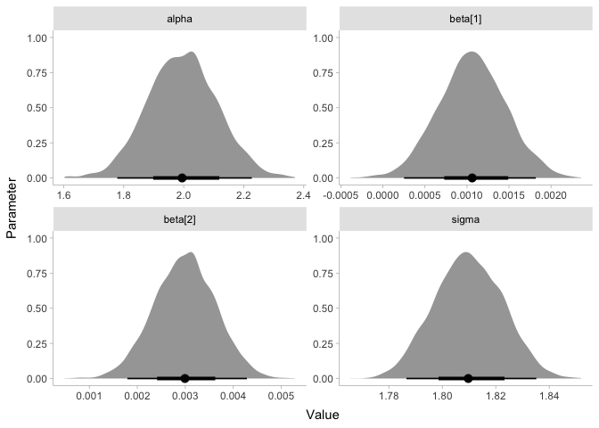
These coefficients might look small, but both beta[1] and beta[2]
appear to exclude 0. Since beta[1] is the coefficient for
duration_s, it says that every one-second increase in the duration of
a track is associated with an increase in .001 * one million = 1000
streams on average! Likewise, beta[2] says that an increase of one
beat per minute of the tempo is associated with an increase of 3000
streams.
Design matrices and you
It looks for sure like there are some effects of duration and tempo on stream counts in the top 200. Could it be that these effects interact with each other? In other words, could the effect of duration depend on tempo? It’s easy to imagine that longer songs could get boring if they are too slow, or perhaps they are overstimulating if they are too fast.
To find out, let’s run one more model. It turns out that we don’t even
need to code a new Stan program, we can use the last one! All we need to
do is set up our input to Stan in a way that allows for interaction
terms. We could do this manually, but there’s a nice trick to do it much
more easily: use the function model.matrix. You can think of
model.matrix as like the lm function, except that it produces a
design matrix X instead of fitting a linear model. It takes a formula
representing the variables to include in your model and a dataframe
including all of the relevant variables, and it produces an N by K
matrix that we can give to Stan. Let’s take a look at our old design
matrix:
1
head(model.matrix(streams ~ duration_s + tempo, data=spotify2021))
1
2
3
4
5
6
7
##   (Intercept) duration_s   tempo
## 1           1    279.204 121.002
## 2           1    190.779 115.884
## 3           1    173.711 109.978
## 4           1    140.526  90.989
## 5           1    195.429 140.042
## 6           1    205.090 109.928
This matrix has a column of one’s for the intercept, a column for
duration_s, a column for tempo, and a column for loudness. But
since we have the intercept alpha defined separately in our model, we
can get rid of the intercept column using the notation 0 + ....
1
head(model.matrix(streams ~ 0 + duration_s + tempo, data=spotify2021))
1
2
3
4
5
6
7
##   duration_s   tempo
## 1    279.204 121.002
## 2    190.779 115.884
## 3    173.711 109.978
## 4    140.526  90.989
## 5    195.429 140.042
## 6    205.090 109.928
Finally, let’s add in an interaction term:
1
2
X <- model.matrix(streams ~ 0 + duration_s * tempo, data=spotify2021)
head(X)
1
2
3
4
5
6
7
##   duration_s   tempo duration_s:tempo
## 1    279.204 121.002         33784.24
## 2    190.779 115.884         22108.23
## 3    173.711 109.978         19104.39
## 4    140.526  90.989         12786.32
## 5    195.429 140.042         27368.27
## 6    205.090 109.928         22545.13
We now have three columns for our three predictor variables, three columns for the two-way interactions, and one column for the three-way interaction. Let’s see what happens when we run the model:
1
2
3
4
5
streams_data <- list(N=nrow(spotify2021), K=ncol(X),
                     X=X, y=spotify2021$streams)
streams_model <- cmdstan_model('2021-12-10-streams-glm.stan')  ## compile the model
streams <- streams_model$sample(data=streams_data)
streams
1
2
3
4
5
6
7
8
9
10
11
12
13
14
15
16
17
18
19
20
21
22
23
24
25
26
27
28
29
30
31
32
33
34
35
36
37
38
39
40
41
42
43
44
45
46
47
48
49
50
51
52
53
54
55
56
57
58
59
60
61
62
63
64
65
66
67
68
69
70
71
72
73
74
75
76
77
78
79
80
81
82
83
84
85
86
87
88
89
90
91
92
93
94
95
96
97
98
99
100
101
102
103
104
105
106
107
108
109
110
111
112
113
114
115
116
117
118
119
120
121
122
## Running MCMC with 4 chains, at most 20 in parallel...
##
## Chain 1 Iteration:    1 / 2000 [  0%]  (Warmup)
## Chain 2 Iteration:    1 / 2000 [  0%]  (Warmup)
## Chain 3 Iteration:    1 / 2000 [  0%]  (Warmup)
## Chain 4 Iteration:    1 / 2000 [  0%]  (Warmup)
## Chain 2 Iteration:  100 / 2000 [  5%]  (Warmup)
## Chain 3 Iteration:  100 / 2000 [  5%]  (Warmup)
## Chain 4 Iteration:  100 / 2000 [  5%]  (Warmup)
## Chain 3 Iteration:  200 / 2000 [ 10%]  (Warmup)
## Chain 4 Iteration:  200 / 2000 [ 10%]  (Warmup)
## Chain 1 Iteration:  100 / 2000 [  5%]  (Warmup)
## Chain 4 Iteration:  300 / 2000 [ 15%]  (Warmup)
## Chain 2 Iteration:  200 / 2000 [ 10%]  (Warmup)
## Chain 3 Iteration:  300 / 2000 [ 15%]  (Warmup)
## Chain 2 Iteration:  300 / 2000 [ 15%]  (Warmup)
## Chain 3 Iteration:  400 / 2000 [ 20%]  (Warmup)
## Chain 4 Iteration:  400 / 2000 [ 20%]  (Warmup)
## Chain 4 Iteration:  500 / 2000 [ 25%]  (Warmup)
## Chain 1 Iteration:  200 / 2000 [ 10%]  (Warmup)
## Chain 2 Iteration:  400 / 2000 [ 20%]  (Warmup)
## Chain 4 Iteration:  600 / 2000 [ 30%]  (Warmup)
## Chain 2 Iteration:  500 / 2000 [ 25%]  (Warmup)
## Chain 3 Iteration:  500 / 2000 [ 25%]  (Warmup)
## Chain 4 Iteration:  700 / 2000 [ 35%]  (Warmup)
## Chain 1 Iteration:  300 / 2000 [ 15%]  (Warmup)
## Chain 2 Iteration:  600 / 2000 [ 30%]  (Warmup)
## Chain 1 Iteration:  400 / 2000 [ 20%]  (Warmup)
## Chain 1 Iteration:  500 / 2000 [ 25%]  (Warmup)
## Chain 4 Iteration:  800 / 2000 [ 40%]  (Warmup)
## Chain 1 Iteration:  600 / 2000 [ 30%]  (Warmup)
## Chain 3 Iteration:  600 / 2000 [ 30%]  (Warmup)
## Chain 4 Iteration:  900 / 2000 [ 45%]  (Warmup)
## Chain 2 Iteration:  700 / 2000 [ 35%]  (Warmup)
## Chain 4 Iteration: 1000 / 2000 [ 50%]  (Warmup)
## Chain 4 Iteration: 1001 / 2000 [ 50%]  (Sampling)
## Chain 3 Iteration:  700 / 2000 [ 35%]  (Warmup)
## Chain 2 Iteration:  800 / 2000 [ 40%]  (Warmup)
## Chain 3 Iteration:  800 / 2000 [ 40%]  (Warmup)
## Chain 2 Iteration:  900 / 2000 [ 45%]  (Warmup)
## Chain 2 Iteration: 1000 / 2000 [ 50%]  (Warmup)
## Chain 2 Iteration: 1001 / 2000 [ 50%]  (Sampling)
## Chain 3 Iteration:  900 / 2000 [ 45%]  (Warmup)
## Chain 2 Iteration: 1100 / 2000 [ 55%]  (Sampling)
## Chain 2 Iteration: 1200 / 2000 [ 60%]  (Sampling)
## Chain 3 Iteration: 1000 / 2000 [ 50%]  (Warmup)
## Chain 3 Iteration: 1001 / 2000 [ 50%]  (Sampling)
## Chain 2 Iteration: 1300 / 2000 [ 65%]  (Sampling)
## Chain 3 Iteration: 1100 / 2000 [ 55%]  (Sampling)
## Chain 2 Iteration: 1400 / 2000 [ 70%]  (Sampling)
## Chain 3 Iteration: 1200 / 2000 [ 60%]  (Sampling)
## Chain 2 Iteration: 1500 / 2000 [ 75%]  (Sampling)
## Chain 2 Iteration: 1600 / 2000 [ 80%]  (Sampling)
## Chain 3 Iteration: 1300 / 2000 [ 65%]  (Sampling)
## Chain 1 Iteration:  700 / 2000 [ 35%]  (Warmup)
## Chain 2 Iteration: 1700 / 2000 [ 85%]  (Sampling)
## Chain 3 Iteration: 1400 / 2000 [ 70%]  (Sampling)
## Chain 4 Iteration: 1100 / 2000 [ 55%]  (Sampling)
## Chain 2 Iteration: 1800 / 2000 [ 90%]  (Sampling)
## Chain 3 Iteration: 1500 / 2000 [ 75%]  (Sampling)
## Chain 2 Iteration: 1900 / 2000 [ 95%]  (Sampling)
## Chain 3 Iteration: 1600 / 2000 [ 80%]  (Sampling)
## Chain 2 Iteration: 2000 / 2000 [100%]  (Sampling)
## Chain 2 finished in 13.0 seconds.
## Chain 3 Iteration: 1700 / 2000 [ 85%]  (Sampling)
## Chain 3 Iteration: 1800 / 2000 [ 90%]  (Sampling)
## Chain 3 Iteration: 1900 / 2000 [ 95%]  (Sampling)
## Chain 3 Iteration: 2000 / 2000 [100%]  (Sampling)
## Chain 3 finished in 15.9 seconds.
## Chain 4 Iteration: 1200 / 2000 [ 60%]  (Sampling)
## Chain 1 Iteration:  800 / 2000 [ 40%]  (Warmup)
## Chain 4 Iteration: 1300 / 2000 [ 65%]  (Sampling)
## Chain 4 Iteration: 1400 / 2000 [ 70%]  (Sampling)
## Chain 1 Iteration:  900 / 2000 [ 45%]  (Warmup)
## Chain 4 Iteration: 1500 / 2000 [ 75%]  (Sampling)
## Chain 1 Iteration: 1000 / 2000 [ 50%]  (Warmup)
## Chain 1 Iteration: 1001 / 2000 [ 50%]  (Sampling)
## Chain 4 Iteration: 1600 / 2000 [ 80%]  (Sampling)
## Chain 4 Iteration: 1700 / 2000 [ 85%]  (Sampling)
## Chain 1 Iteration: 1100 / 2000 [ 55%]  (Sampling)
## Chain 4 Iteration: 1800 / 2000 [ 90%]  (Sampling)
## Chain 4 Iteration: 1900 / 2000 [ 95%]  (Sampling)
## Chain 1 Iteration: 1200 / 2000 [ 60%]  (Sampling)
## Chain 4 Iteration: 2000 / 2000 [100%]  (Sampling)
## Chain 4 finished in 84.1 seconds.
## Chain 1 Iteration: 1300 / 2000 [ 65%]  (Sampling)
## Chain 1 Iteration: 1400 / 2000 [ 70%]  (Sampling)
## Chain 1 Iteration: 1500 / 2000 [ 75%]  (Sampling)
## Chain 1 Iteration: 1600 / 2000 [ 80%]  (Sampling)
## Chain 1 Iteration: 1700 / 2000 [ 85%]  (Sampling)
## Chain 1 Iteration: 1800 / 2000 [ 90%]  (Sampling)
## Chain 1 Iteration: 1900 / 2000 [ 95%]  (Sampling)
## Chain 1 Iteration: 2000 / 2000 [100%]  (Sampling)
## Chain 1 finished in 193.7 seconds.
##
## All 4 chains finished successfully.
## Mean chain execution time: 76.7 seconds.
## Total execution time: 193.8 seconds.
##  variable      mean    median     sd   mad        q5       q95 rhat ess_bulk
##   lp__    -10420.09 -10276.90 490.69 10.23 -10679.73 -10269.10 2.15        5
##   alpha        0.72      1.24   1.25  0.45     -1.40      1.82 3.37        4
##   beta[1]      0.01      0.01   0.01  0.00      0.00      0.02 2.43        4
##   beta[2]      0.01      0.01   0.01  0.00      0.01      0.03 2.43        4
##   beta[3]      0.00      0.00   0.00  0.00      0.00      0.00 2.41        4
##   sigma        1.95      1.83   0.32  0.04      1.79      2.25 2.14        5
##   mu[1]        2.63      2.63   0.06  0.04      2.56      2.71 1.13       20
##   mu[2]        2.54      2.55   0.03  0.02      2.50      2.58 1.26       11
##   mu[3]        2.50      2.51   0.05  0.04      2.42      2.56 1.66        6
##   mu[4]        2.34      2.38   0.14  0.07      2.10      2.48 2.19        5
##  ess_tail
##        18
##         8
##        38
##        29
##        28
##        18
##        44
##        31
##        26
##        29
##
##  # showing 10 of 18806 rows (change via 'max_rows' argument or 'cmdstanr_max_rows' option)
Ah, the model has yet again failed to converge. Looking at the above
design matrix, it looks like a similar thing could be going on: the
interaction variable seems to be much larger than the two other
variables. This makes sense, because interactions are just
multiplications of other variables (the data for duration_s:tempo is
just duration_s * tempo). So what can we do? Well, we have a couple
options. As we mentioned before, we could z-score our variables. But as
we mentioned before, that removes all of the information about the
scales, which makes it hard to tell the size of the effects. So we’re
going to scale down both duration (to minutes) and tempo (to beats
per second) individually to make sure that the interaction doesn’t blow
out of proportion.
1
2
3
4
5
6
7
8
9
10
spotify2021$duration_m <- spotify2021$duration_s / 60
spotify2021$tempo_bps <- spotify2021$tempo / 60

X <- model.matrix(streams ~ 0 + duration_m * tempo_bps, data=spotify2021)
head(X)

streams_data <- list(N=nrow(spotify2021), K=ncol(X),
                     X=X, y=spotify2021$streams)
streams <- streams_model$sample(data=streams_data)
streams
1
2
3
4
5
6
7
8
9
10
11
12
13
14
15
16
17
18
19
20
21
22
23
24
25
26
27
28
29
30
31
32
33
34
35
36
37
38
39
40
41
42
43
44
45
46
47
48
49
50
51
52
53
54
55
56
57
58
59
60
61
62
63
64
65
66
67
68
69
70
71
72
73
74
75
76
77
78
79
80
81
82
83
84
85
86
87
88
89
90
91
92
93
94
95
96
97
98
99
100
101
102
103
104
105
106
107
108
109
110
111
112
113
114
115
116
117
118
119
120
121
122
123
124
125
126
127
128
129
##   duration_m tempo_bps duration_m:tempo_bps
## 1   4.653400  2.016700             9.384512
## 2   3.179650  1.931400             6.141176
## 3   2.895183  1.832967             5.306775
## 4   2.342100  1.516483             3.551756
## 5   3.257150  2.334033             7.602297
## 6   3.418167  1.832133             6.262537
## Running MCMC with 4 chains, at most 20 in parallel...
##
## Chain 1 Iteration:    1 / 2000 [  0%]  (Warmup)
## Chain 2 Iteration:    1 / 2000 [  0%]  (Warmup)
## Chain 3 Iteration:    1 / 2000 [  0%]  (Warmup)
## Chain 4 Iteration:    1 / 2000 [  0%]  (Warmup)
## Chain 1 Iteration:  100 / 2000 [  5%]  (Warmup)
## Chain 2 Iteration:  100 / 2000 [  5%]  (Warmup)
## Chain 4 Iteration:  100 / 2000 [  5%]  (Warmup)
## Chain 3 Iteration:  100 / 2000 [  5%]  (Warmup)
## Chain 2 Iteration:  200 / 2000 [ 10%]  (Warmup)
## Chain 3 Iteration:  200 / 2000 [ 10%]  (Warmup)
## Chain 4 Iteration:  200 / 2000 [ 10%]  (Warmup)
## Chain 1 Iteration:  200 / 2000 [ 10%]  (Warmup)
## Chain 2 Iteration:  300 / 2000 [ 15%]  (Warmup)
## Chain 1 Iteration:  300 / 2000 [ 15%]  (Warmup)
## Chain 3 Iteration:  300 / 2000 [ 15%]  (Warmup)
## Chain 4 Iteration:  300 / 2000 [ 15%]  (Warmup)
## Chain 2 Iteration:  400 / 2000 [ 20%]  (Warmup)
## Chain 1 Iteration:  400 / 2000 [ 20%]  (Warmup)
## Chain 3 Iteration:  400 / 2000 [ 20%]  (Warmup)
## Chain 4 Iteration:  400 / 2000 [ 20%]  (Warmup)
## Chain 2 Iteration:  500 / 2000 [ 25%]  (Warmup)
## Chain 1 Iteration:  500 / 2000 [ 25%]  (Warmup)
## Chain 3 Iteration:  500 / 2000 [ 25%]  (Warmup)
## Chain 4 Iteration:  500 / 2000 [ 25%]  (Warmup)
## Chain 1 Iteration:  600 / 2000 [ 30%]  (Warmup)
## Chain 2 Iteration:  600 / 2000 [ 30%]  (Warmup)
## Chain 3 Iteration:  600 / 2000 [ 30%]  (Warmup)
## Chain 4 Iteration:  600 / 2000 [ 30%]  (Warmup)
## Chain 1 Iteration:  700 / 2000 [ 35%]  (Warmup)
## Chain 2 Iteration:  700 / 2000 [ 35%]  (Warmup)
## Chain 4 Iteration:  700 / 2000 [ 35%]  (Warmup)
## Chain 3 Iteration:  700 / 2000 [ 35%]  (Warmup)
## Chain 1 Iteration:  800 / 2000 [ 40%]  (Warmup)
## Chain 4 Iteration:  800 / 2000 [ 40%]  (Warmup)
## Chain 2 Iteration:  800 / 2000 [ 40%]  (Warmup)
## Chain 3 Iteration:  800 / 2000 [ 40%]  (Warmup)
## Chain 1 Iteration:  900 / 2000 [ 45%]  (Warmup)
## Chain 4 Iteration:  900 / 2000 [ 45%]  (Warmup)
## Chain 3 Iteration:  900 / 2000 [ 45%]  (Warmup)
## Chain 2 Iteration:  900 / 2000 [ 45%]  (Warmup)
## Chain 1 Iteration: 1000 / 2000 [ 50%]  (Warmup)
## Chain 1 Iteration: 1001 / 2000 [ 50%]  (Sampling)
## Chain 3 Iteration: 1000 / 2000 [ 50%]  (Warmup)
## Chain 2 Iteration: 1000 / 2000 [ 50%]  (Warmup)
## Chain 3 Iteration: 1001 / 2000 [ 50%]  (Sampling)
## Chain 2 Iteration: 1001 / 2000 [ 50%]  (Sampling)
## Chain 4 Iteration: 1000 / 2000 [ 50%]  (Warmup)
## Chain 4 Iteration: 1001 / 2000 [ 50%]  (Sampling)
## Chain 1 Iteration: 1100 / 2000 [ 55%]  (Sampling)
## Chain 3 Iteration: 1100 / 2000 [ 55%]  (Sampling)
## Chain 2 Iteration: 1100 / 2000 [ 55%]  (Sampling)
## Chain 4 Iteration: 1100 / 2000 [ 55%]  (Sampling)
## Chain 3 Iteration: 1200 / 2000 [ 60%]  (Sampling)
## Chain 1 Iteration: 1200 / 2000 [ 60%]  (Sampling)
## Chain 2 Iteration: 1200 / 2000 [ 60%]  (Sampling)
## Chain 4 Iteration: 1200 / 2000 [ 60%]  (Sampling)
## Chain 3 Iteration: 1300 / 2000 [ 65%]  (Sampling)
## Chain 1 Iteration: 1300 / 2000 [ 65%]  (Sampling)
## Chain 2 Iteration: 1300 / 2000 [ 65%]  (Sampling)
## Chain 4 Iteration: 1300 / 2000 [ 65%]  (Sampling)
## Chain 3 Iteration: 1400 / 2000 [ 70%]  (Sampling)
## Chain 1 Iteration: 1400 / 2000 [ 70%]  (Sampling)
## Chain 2 Iteration: 1400 / 2000 [ 70%]  (Sampling)
## Chain 4 Iteration: 1400 / 2000 [ 70%]  (Sampling)
## Chain 3 Iteration: 1500 / 2000 [ 75%]  (Sampling)
## Chain 1 Iteration: 1500 / 2000 [ 75%]  (Sampling)
## Chain 2 Iteration: 1500 / 2000 [ 75%]  (Sampling)
## Chain 3 Iteration: 1600 / 2000 [ 80%]  (Sampling)
## Chain 4 Iteration: 1500 / 2000 [ 75%]  (Sampling)
## Chain 1 Iteration: 1600 / 2000 [ 80%]  (Sampling)
## Chain 2 Iteration: 1600 / 2000 [ 80%]  (Sampling)
## Chain 3 Iteration: 1700 / 2000 [ 85%]  (Sampling)
## Chain 4 Iteration: 1600 / 2000 [ 80%]  (Sampling)
## Chain 1 Iteration: 1700 / 2000 [ 85%]  (Sampling)
## Chain 3 Iteration: 1800 / 2000 [ 90%]  (Sampling)
## Chain 2 Iteration: 1700 / 2000 [ 85%]  (Sampling)
## Chain 4 Iteration: 1700 / 2000 [ 85%]  (Sampling)
## Chain 1 Iteration: 1800 / 2000 [ 90%]  (Sampling)
## Chain 3 Iteration: 1900 / 2000 [ 95%]  (Sampling)
## Chain 2 Iteration: 1800 / 2000 [ 90%]  (Sampling)
## Chain 4 Iteration: 1800 / 2000 [ 90%]  (Sampling)
## Chain 3 Iteration: 2000 / 2000 [100%]  (Sampling)
## Chain 3 finished in 32.4 seconds.
## Chain 1 Iteration: 1900 / 2000 [ 95%]  (Sampling)
## Chain 2 Iteration: 1900 / 2000 [ 95%]  (Sampling)
## Chain 4 Iteration: 1900 / 2000 [ 95%]  (Sampling)
## Chain 1 Iteration: 2000 / 2000 [100%]  (Sampling)
## Chain 1 finished in 34.5 seconds.
## Chain 2 Iteration: 2000 / 2000 [100%]  (Sampling)
## Chain 2 finished in 35.3 seconds.
## Chain 4 Iteration: 2000 / 2000 [100%]  (Sampling)
## Chain 4 finished in 36.2 seconds.
##
## All 4 chains finished successfully.
## Mean chain execution time: 34.6 seconds.
## Total execution time: 36.3 seconds.
##  variable      mean    median   sd  mad        q5       q95 rhat ess_bulk
##   lp__    -10269.61 -10269.30 1.58 1.48 -10272.60 -10267.70 1.00     1112
##   alpha        0.66      0.67 0.31 0.30      0.12      1.16 1.00      541
##   beta[1]      0.47      0.46 0.09 0.09      0.32      0.62 1.00      533
##   beta[2]      0.86      0.86 0.15 0.15      0.62      1.13 1.00      528
##   beta[3]     -0.21     -0.20 0.05 0.04     -0.29     -0.14 1.00      523
##   sigma        1.81      1.81 0.01 0.01      1.79      1.83 1.00     1599
##   mu[1]        2.63      2.63 0.04 0.04      2.57      2.69 1.00     4441
##   mu[2]        2.54      2.54 0.02 0.02      2.51      2.57 1.00     4013
##   mu[3]        2.50      2.50 0.02 0.02      2.46      2.54 1.00     3525
##   mu[4]        2.33      2.33 0.04 0.04      2.26      2.39 1.00     1421
##  ess_tail
##      1327
##       630
##       671
##       700
##       733
##      1615
##      3322
##      3168
##      2544
##      1970
##
##  # showing 10 of 18806 rows (change via 'max_rows' argument or 'cmdstanr_max_rows' option)
It’s not perfect, but for our purposes it’ll do just fine. Let’s plot our parameters:
1
2
3
4
5
6
7
streams$draws(c('alpha', 'beta', 'sigma'), format='draws_df') %>%
    pivot_longer(alpha:sigma, names_to='.variable', values_to='.value') %>%
    ggplot(aes(x=.value)) +
    stat_halfeye(point_interval=median_hdi, normalize='panels') +
    xlab('Value') + ylab('Parameter') +
    facet_wrap(~ .variable, scales='free') +
    theme_tidybayes()
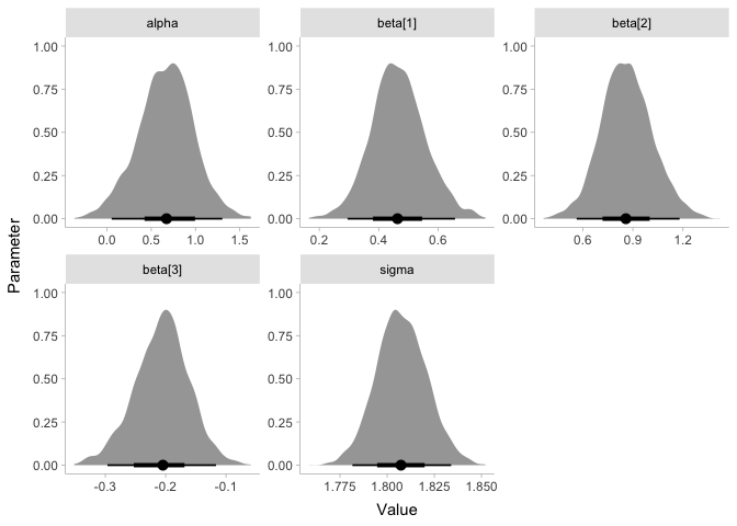
From our model’s results, it looks like we do indeed have a negative
interaction: even though stream counts go up by about 450,000 with each
additional minute (beta[1]), and even though they go up by about
850,000 for each beat-per-second increase in tempo (beta[2]), these
relationships reverse if a song is either too long or too fast. To
visualize how this relationships change, we can add to our Stan program
to calculate model predictions for any arbitrary X:
1
2
3
4
5
6
7
8
9
10
11
12
13
14
15
16
17
18
19
20
21
22
23
24
25
26
27
28
29
30
31
32
33
34
data {
  int<lower=0> N;      // the number of data points
  int<lower=0> K;      // the number of regression coefficients
  matrix[N, K] X;      // the predictor variables
  vector[N] y;         // the outcome variable

  int<lower=0> N_pred;        // the number of prediction points
  matrix[N_pred, K] X_pred;   // the prediction points
}

parameters {
  real alpha;
  vector[K] beta;
  real<lower=0> sigma;
}

transformed parameters {
  vector[N] mu = alpha + X*beta;
}

model {
  alpha ~ normal(0, 1);
  beta ~ normal(0, 1);
  sigma ~ normal(0, 1);

  y ~ normal(mu, sigma);
}

generated quantities {
  real y_hat[N] = normal_rng(mu, sigma);

  vector[N_pred] mu_pred = alpha + X_pred*beta;
  real y_pred_hat[N_pred] = normal_rng(mu_pred, sigma);
}
Now in addition to X, we’re also giving Stan a different dataset
called X_pred, which contains some values of the predictors we want
model predictions for. Since this data isn’t involved in training, we
don’t need a corresponding y_pred. In the generated quantities, I’ve
added two new variables. mu_pred is the model prediction for the mean
of y at X_pred, and y_pred_hat are the simulated data at X_pred.
Let’s try it out:
1
2
3
4
5
6
7
8
9
10
11
X_pred <- expand_grid(duration_m=seq(0, 10, 1),
                      tempo_bps=seq(0.5, 3, 0.5)) %>%
    model.matrix( ~ 0 + duration_m * tempo_bps, .)
head(X_pred)

streams_data <- list(N=nrow(spotify2021), K=ncol(X),
                     X=X, y=spotify2021$streams,
                     N_pred=nrow(X_pred), X_pred=X_pred)
streams_model <- cmdstan_model('2021-12-10-streams-glm-pred.stan')
streams <- streams_model$sample(data=streams_data)
streams
1
2
3
4
5
6
7
8
9
10
11
12
13
14
15
16
17
18
19
20
21
22
23
24
25
26
27
28
29
30
31
32
33
34
35
36
37
38
39
40
41
42
43
44
45
46
47
48
49
50
51
52
53
54
55
56
57
58
59
60
61
62
63
64
65
66
67
68
69
70
71
72
73
74
75
76
77
78
79
80
81
82
83
84
85
86
87
88
89
90
91
92
93
94
95
96
97
98
99
100
101
102
103
104
105
106
107
108
109
110
111
112
113
114
115
116
117
118
119
120
121
122
123
124
125
126
127
128
129
##   duration_m tempo_bps duration_m:tempo_bps
## 1          0       0.5                    0
## 2          0       1.0                    0
## 3          0       1.5                    0
## 4          0       2.0                    0
## 5          0       2.5                    0
## 6          0       3.0                    0
## Running MCMC with 4 chains, at most 20 in parallel...
##
## Chain 1 Iteration:    1 / 2000 [  0%]  (Warmup)
## Chain 2 Iteration:    1 / 2000 [  0%]  (Warmup)
## Chain 3 Iteration:    1 / 2000 [  0%]  (Warmup)
## Chain 4 Iteration:    1 / 2000 [  0%]  (Warmup)
## Chain 1 Iteration:  100 / 2000 [  5%]  (Warmup)
## Chain 1 Iteration:  200 / 2000 [ 10%]  (Warmup)
## Chain 1 Iteration:  300 / 2000 [ 15%]  (Warmup)
## Chain 2 Iteration:  100 / 2000 [  5%]  (Warmup)
## Chain 2 Iteration:  200 / 2000 [ 10%]  (Warmup)
## Chain 2 Iteration:  300 / 2000 [ 15%]  (Warmup)
## Chain 3 Iteration:  100 / 2000 [  5%]  (Warmup)
## Chain 3 Iteration:  200 / 2000 [ 10%]  (Warmup)
## Chain 3 Iteration:  300 / 2000 [ 15%]  (Warmup)
## Chain 4 Iteration:  100 / 2000 [  5%]  (Warmup)
## Chain 4 Iteration:  200 / 2000 [ 10%]  (Warmup)
## Chain 4 Iteration:  300 / 2000 [ 15%]  (Warmup)
## Chain 2 Iteration:  400 / 2000 [ 20%]  (Warmup)
## Chain 3 Iteration:  400 / 2000 [ 20%]  (Warmup)
## Chain 4 Iteration:  400 / 2000 [ 20%]  (Warmup)
## Chain 1 Iteration:  400 / 2000 [ 20%]  (Warmup)
## Chain 2 Iteration:  500 / 2000 [ 25%]  (Warmup)
## Chain 1 Iteration:  500 / 2000 [ 25%]  (Warmup)
## Chain 3 Iteration:  500 / 2000 [ 25%]  (Warmup)
## Chain 4 Iteration:  500 / 2000 [ 25%]  (Warmup)
## Chain 2 Iteration:  600 / 2000 [ 30%]  (Warmup)
## Chain 1 Iteration:  600 / 2000 [ 30%]  (Warmup)
## Chain 3 Iteration:  600 / 2000 [ 30%]  (Warmup)
## Chain 2 Iteration:  700 / 2000 [ 35%]  (Warmup)
## Chain 4 Iteration:  600 / 2000 [ 30%]  (Warmup)
## Chain 1 Iteration:  700 / 2000 [ 35%]  (Warmup)
## Chain 3 Iteration:  700 / 2000 [ 35%]  (Warmup)
## Chain 2 Iteration:  800 / 2000 [ 40%]  (Warmup)
## Chain 4 Iteration:  700 / 2000 [ 35%]  (Warmup)
## Chain 1 Iteration:  800 / 2000 [ 40%]  (Warmup)
## Chain 2 Iteration:  900 / 2000 [ 45%]  (Warmup)
## Chain 3 Iteration:  800 / 2000 [ 40%]  (Warmup)
## Chain 4 Iteration:  800 / 2000 [ 40%]  (Warmup)
## Chain 3 Iteration:  900 / 2000 [ 45%]  (Warmup)
## Chain 1 Iteration:  900 / 2000 [ 45%]  (Warmup)
## Chain 2 Iteration: 1000 / 2000 [ 50%]  (Warmup)
## Chain 2 Iteration: 1001 / 2000 [ 50%]  (Sampling)
## Chain 4 Iteration:  900 / 2000 [ 45%]  (Warmup)
## Chain 3 Iteration: 1000 / 2000 [ 50%]  (Warmup)
## Chain 3 Iteration: 1001 / 2000 [ 50%]  (Sampling)
## Chain 1 Iteration: 1000 / 2000 [ 50%]  (Warmup)
## Chain 1 Iteration: 1001 / 2000 [ 50%]  (Sampling)
## Chain 4 Iteration: 1000 / 2000 [ 50%]  (Warmup)
## Chain 4 Iteration: 1001 / 2000 [ 50%]  (Sampling)
## Chain 2 Iteration: 1100 / 2000 [ 55%]  (Sampling)
## Chain 1 Iteration: 1100 / 2000 [ 55%]  (Sampling)
## Chain 3 Iteration: 1100 / 2000 [ 55%]  (Sampling)
## Chain 4 Iteration: 1100 / 2000 [ 55%]  (Sampling)
## Chain 2 Iteration: 1200 / 2000 [ 60%]  (Sampling)
## Chain 1 Iteration: 1200 / 2000 [ 60%]  (Sampling)
## Chain 3 Iteration: 1200 / 2000 [ 60%]  (Sampling)
## Chain 4 Iteration: 1200 / 2000 [ 60%]  (Sampling)
## Chain 2 Iteration: 1300 / 2000 [ 65%]  (Sampling)
## Chain 1 Iteration: 1300 / 2000 [ 65%]  (Sampling)
## Chain 3 Iteration: 1300 / 2000 [ 65%]  (Sampling)
## Chain 4 Iteration: 1300 / 2000 [ 65%]  (Sampling)
## Chain 2 Iteration: 1400 / 2000 [ 70%]  (Sampling)
## Chain 1 Iteration: 1400 / 2000 [ 70%]  (Sampling)
## Chain 3 Iteration: 1400 / 2000 [ 70%]  (Sampling)
## Chain 4 Iteration: 1400 / 2000 [ 70%]  (Sampling)
## Chain 1 Iteration: 1500 / 2000 [ 75%]  (Sampling)
## Chain 2 Iteration: 1500 / 2000 [ 75%]  (Sampling)
## Chain 3 Iteration: 1500 / 2000 [ 75%]  (Sampling)
## Chain 4 Iteration: 1500 / 2000 [ 75%]  (Sampling)
## Chain 1 Iteration: 1600 / 2000 [ 80%]  (Sampling)
## Chain 2 Iteration: 1600 / 2000 [ 80%]  (Sampling)
## Chain 3 Iteration: 1600 / 2000 [ 80%]  (Sampling)
## Chain 4 Iteration: 1600 / 2000 [ 80%]  (Sampling)
## Chain 1 Iteration: 1700 / 2000 [ 85%]  (Sampling)
## Chain 2 Iteration: 1700 / 2000 [ 85%]  (Sampling)
## Chain 3 Iteration: 1700 / 2000 [ 85%]  (Sampling)
## Chain 4 Iteration: 1700 / 2000 [ 85%]  (Sampling)
## Chain 2 Iteration: 1800 / 2000 [ 90%]  (Sampling)
## Chain 1 Iteration: 1800 / 2000 [ 90%]  (Sampling)
## Chain 3 Iteration: 1800 / 2000 [ 90%]  (Sampling)
## Chain 4 Iteration: 1800 / 2000 [ 90%]  (Sampling)
## Chain 1 Iteration: 1900 / 2000 [ 95%]  (Sampling)
## Chain 2 Iteration: 1900 / 2000 [ 95%]  (Sampling)
## Chain 3 Iteration: 1900 / 2000 [ 95%]  (Sampling)
## Chain 4 Iteration: 1900 / 2000 [ 95%]  (Sampling)
## Chain 1 Iteration: 2000 / 2000 [100%]  (Sampling)
## Chain 1 finished in 34.0 seconds.
## Chain 2 Iteration: 2000 / 2000 [100%]  (Sampling)
## Chain 2 finished in 34.3 seconds.
## Chain 3 Iteration: 2000 / 2000 [100%]  (Sampling)
## Chain 3 finished in 35.8 seconds.
## Chain 4 Iteration: 2000 / 2000 [100%]  (Sampling)
## Chain 4 finished in 35.8 seconds.
##
## All 4 chains finished successfully.
## Mean chain execution time: 35.0 seconds.
## Total execution time: 35.9 seconds.
##  variable      mean    median   sd  mad        q5       q95 rhat ess_bulk
##   lp__    -10269.62 -10269.30 1.57 1.48 -10272.60 -10267.70 1.00     1285
##   alpha        0.67      0.67 0.31 0.30      0.15      1.19 1.01      683
##   beta[1]      0.46      0.46 0.09 0.09      0.31      0.62 1.01      688
##   beta[2]      0.86      0.86 0.15 0.15      0.60      1.11 1.01      680
##   beta[3]     -0.21     -0.20 0.04 0.04     -0.28     -0.13 1.01      690
##   sigma        1.81      1.81 0.01 0.01      1.79      1.83 1.00     1578
##   mu[1]        2.63      2.63 0.04 0.04      2.57      2.70 1.00     4807
##   mu[2]        2.54      2.54 0.02 0.02      2.51      2.58 1.00     4563
##   mu[3]        2.50      2.50 0.02 0.02      2.46      2.54 1.00     3801
##   mu[4]        2.33      2.33 0.04 0.04      2.26      2.40 1.00     1556
##  ess_tail
##      1905
##       908
##       923
##       835
##       794
##      1568
##      3453
##      3361
##      3323
##      2485
##
##  # showing 10 of 18938 rows (change via 'max_rows' argument or 'cmdstanr_max_rows' option)
Thankfully, the results are pretty much the same. Let’s see what those predictions look like!
1
2
3
4
5
6
7
8
9
10
11
12
13
14
15
streams %>%
    spread_draws(mu_pred[.row]) %>%
    mutate(duration_m=X_pred[.row, 'duration_m'],
           tempo_bps=X_pred[.row, 'tempo_bps']) %>%
    group_by(duration_m, tempo_bps) %>%
    median_hdi %>%
    ggplot(aes(x=duration_m, y=mu_pred, group=tempo_bps, fill=tempo_bps)) +
    geom_point(aes(y=streams, color=tempo_bps), alpha=.25, size=.25, data=spotify2021) +
    geom_ribbon(aes(ymin=.lower, ymax=.upper), alpha=.25) +
    geom_line(aes(color=tempo_bps)) +
    xlab('Duration (minutes)') + ylab('Streams (millions)') +
    scale_color_viridis(name='Tempo\n(beats/second)') +
    scale_fill_viridis(name='Tempo\n(beats/second)') +
    coord_cartesian(xlim=c(1, 6), ylim=c(0, 5)) +
    theme_tidybayes()
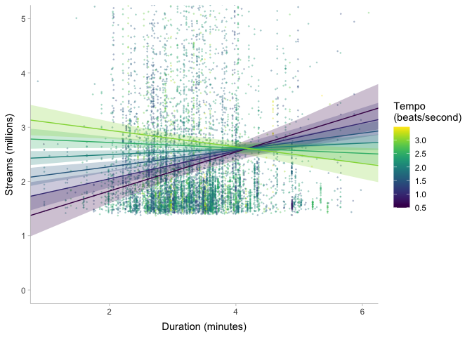
We can see the overall trends we found earlier: for slower songs, there is a positive relationship between duration and stream count, but for faster songs this trend is reversed (with the switch from positive to negative happening around 2 beats/second). Most importantly, though, our model doesn’t seem to be describing the data super well. If our goal is just to describe some overall patterns in the data, our current model is probably fine. But if we are interested in capturing the data-generating process of stream counts, then we would probably want to refine this model some more until the model-generated data looks reasonably like the actual data.
Summary
In this tutorial, we learned what probabilistic programming is, and we walked through some of the many ways in which you can use the probabilistic programming language Stan. We simulated fake data from a model, simulated fake data from a prior distribution, fit a few different linear models to some data, and visualized linear trends in the data! Although this is a lot, there’s so much more that you can do with Stan, so expect to see it in more tutorials to come. Until next time!