Why are we even here?

We, crazy neuroscientists, study the brain with the hope of ultimately being able to read one’s every single thought and manipulate them. With the power of neuroimaging techiniques and money, we get to experiment on willing participants and measure some type of physiological changes which are associated with the brain’s (ab)normal functioning.

Assuming we want to save the world by understanding how the brain differentiates two categories: animals (cats, pandas, dolphins, T-rexes) and vehicles (scooters, tractors, submarines, spacecrafts), and we happen to have a blood oxygenation level dependent (BOLD) functional magnetic resonance imaging (fMRI) scanner at our disposal, here’s what we could do:

1. Get money.
2. Use money (and force, if necessary) to get subjects.
3. Show a series of pictures of both animals and vehicles, while BOLD fMRI measures the change in the proportion of oxygenated haemoglobin in the blood flow in the brain, a proxy for brain activity.
4. Check data quality and preprocess data.
5. Model subject-level data with general linear models (GLMs), which will estimate how much (expressed as βs) the increase/decrease in brain activity is due to each event (e.g., image presentation, button press, subjects’ screaming for experiment termination).

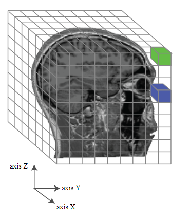
source: http://gureckislab.org/courses/fall19/labincp/labs/lab1mri-pt1.html

Because of the data aquisition style of fMRI, brains are parcelated into voxels–the smallest unit of (meaningful) data, commonly 3mm x 3mm x 3mm in size. Assuming all went well, we get people’s brain activity pattern for their viewing of each picture. The data structure for each subject can be thought of a giant matrix with

100,000 (voxels) x 2 (categories) x 60 (items) entries of β estimates. 

With some vague knowledge of brain anatomy, we remember several different interesting regions in the brain such as the hippocampus, the amygdala, and the ventricles, and we decide to look at these regions-of-interest (ROIs).

Assuming that each ROI is homogeneous (i.e., engagement is uniform throughout), we can take the average of βs across all voxels within each ROI, and get an ROI-level matrix with

2 (categories) x 60 (items) entries of averaged β estimates.

Now we can perform a two-sample t-test to compare which category–animals or vehicles–elicited greater brain activation in our favorite ROI, the ventricles, and start writing our Nobel Prize acceptance speech.

1
2
3
4
% obviously fake data
beta_animals = 0.5 + randn(1, 60);
beta_vehicles = 0.0 + randn(1, 60);
[h,p,ci,stat] = ttest2(beta_animals, beta_vehicles)

h = 1
p = 0.0321
ci = 1x2    
    0.0360    0.7924

stat = 
    tstat: 2.1686
       df: 118
       sd: 1.0461

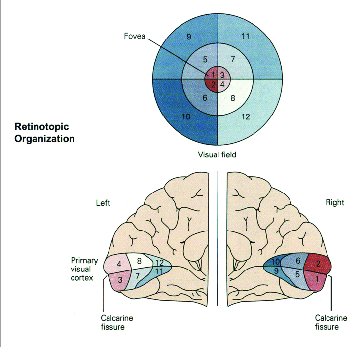
The analysis we just went through is commonly referred to as univariate, because we only cared about and tested on one central variable–the averaged activation level. Univariate analysis is good in terms of signal-to-noise ratios and its clearly defined and easily interpretable contrasts. However, a big assumption of univariate analysis is the the homogeneity of the ROI, with all of its voxels contributing to just one signal–not true for the retinotopically organized primary visual cortex (V1).

source: https://www.researchgate.net/figure/Retinotopic-organization-of-the-primary-visual-cortex-Up-to-50-of-the-primary-visual_fig4_325718113

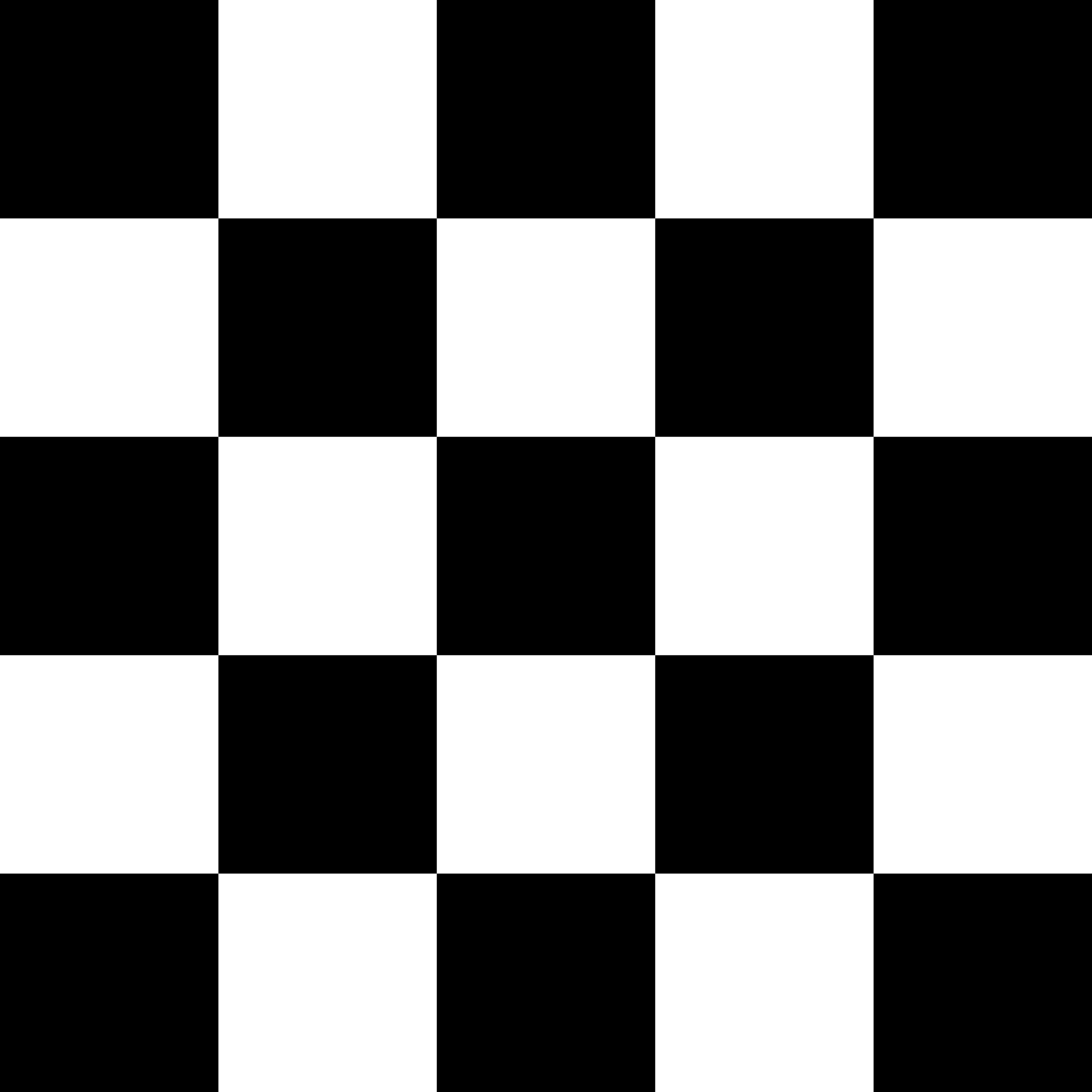
Let’s say we, aspiring neuroscientists, take on a slightly less exciting side project on checkerboards, and we have two checkerboard patterns which have the exact opposite… pattern. We may want to see if V1 has different activation levels in response to the two patterns by conducting a univariate analysis.

1
2
3
4
5
6
7
8
% even more fake data
beta_pattern_A = repmat([1; 2; 3; 4], 25, 60) + randn(100, 60) * 0.1;
beta_pattern_B = repmat([3; 1; 4; 2], 25, 60) + randn(100, 60) * 0.1;

% if we do univarite analysis on the averaged patterns...
beta_univ_A = mean(beta_pattern_A, 1);
beta_univ_B = mean(beta_pattern_B, 1);
[h,p,ci,stat] = ttest2(beta_univ_A, beta_univ_B)

h = 0
p = 0.1116
ci = 1x2    
   -0.0055    0.0006

stat = 
    tstat: -1.6031
       df: 118
       sd: 0.0084

Presumably half of the V1 voxels will correspond a white square and the other half, a black square; that neural pattern is probably reversed for checkerboards A and B, but averaging the activation level across all V1 voxels will just smear the pattern. So, what now?

Enter Multivariate Pattern Analysis

Multivariate pattern analysis (MVPA), also referred to as multivoxel pattern analysis in the context of fMRI, takes advantage of the high spatial resolution of fMRI; instead of assuming just one signal being represented in all voxels within an ROI, MVPA treats the many voxels as a pattern and assumes that information is stored in that pattern.

But then we are faced with another problem: how do we go about analyzing the pattern? Now that each voxels is a variable, and an ROI easily contains hundreds of voxels, the good old t-test just does not help. We will go over two main types of MVPA: decoding analysis and representational similarity analysis (RSA), which resolves that problem differently.

Decoding analyis

Because it is hard to simultaneously test on the multivariate neural patterns, decoding analysis (classification or regression) simply reverses the direction of inference: instead of comparing neural patterns between conditions (e.g., animals vs. vehicles), we can try to decode the conditions from the neural patterns. This reversal can potentially make things easier because the number of conditons is most often way smaller than the number of variables–voxels in the context of fMRI. In order to do that, some computer science-minded people might just say, “machine learning is all you need!”

(If you’re new to machine learning, this DIBS Methods Meetings series is all you need–check out Miles’s nice tutorial on Machine Learning Basics; if you’re feeling fancy, check out this one on Neural Networks).

Because we know the conditions which each experimental trial/block/participant is subjected to–unless we made the huge mistake of not recording those information or a flood or fire destroyed our hard drives, we have a labelled dataset that is suitable for supervised learning. Here we will use a simple classification method named the Support Vector Machine (SVM).

1
2
3
4
5
6
7
8
9
10
11
12
13
14
15
16
17
18
19
20
21
22
23
% sklearn toolbox for MATLAB
% URL: https://www.mathworks.com/matlabcentral/fileexchange/59453-sklearn-matlab
% Note that sklearn is much better developed for Python users, but this MATLAB implementation is sufficient for our purposes.
addpath(genpath('C:\Users\hhh\OneDrive - Duke University\Duke\Research\Resources\sklearn-matlab-master'));

% same old fake data, but more noise
beta_pattern_A = repmat([1; 0], 50, 60) + randn(100, 60) * 4;
beta_pattern_B = repmat([0; 1], 50, 60) + randn(100, 60) * 4;

test_ind = randperm(60, 10); % randomly select test data
train_ind = setdiff(1:60, test_ind); % the rest will be training data

X_train = vertcat(beta_pattern_A(:, train_ind)', beta_pattern_B(:, train_ind)');
X_test = vertcat(beta_pattern_A(:, test_ind)', beta_pattern_B(:, test_ind)');
y_train = [ones(length(train_ind), 1); zeros(length(train_ind), 1)]; % labels; animals = 1, vehicles = 0
y_test = [ones(length(test_ind), 1); zeros(length(test_ind), 1)]; % labels

% clf = SVC(struct('kernel', 'RBF')); % define classifer type
clf = SVC(struct('kernel', 'linear')); % define classifer type
clf.fit(X_train, y_train); % training
y_pred = clf.predict(X_test); % testing
score = accuracy_score(y_test, y_pred); % classification accuracy
fprintf('Accuracy: %.2f%%\n', score*100);

Accuracy: 85.00%

1
2
3
4
5
6
7
8
9
10
11
% make plot on training set
sv = clf.model.SupportVectors;
figure; hold all
ind1 = find(y_train==1);
ind0 = find(y_train==0);
plot(X_train(ind1, 1), X_train(ind1, 2),'.','MarkerSize',16)
plot(X_train(ind0, 1), X_train(ind0, 2),'.','MarkerSize',16)
plot(sv(:,1),sv(:,2),'ko','MarkerSize',5)
title(sprintf("This doesn't look separable at %.2f%% accuracy... Why?", score*100))
legend({'Animals','Vehicles','Support Vector'},'Location','best')
set(gca, 'Units','normalized','Position', [.1 .4 .8 .5]); 

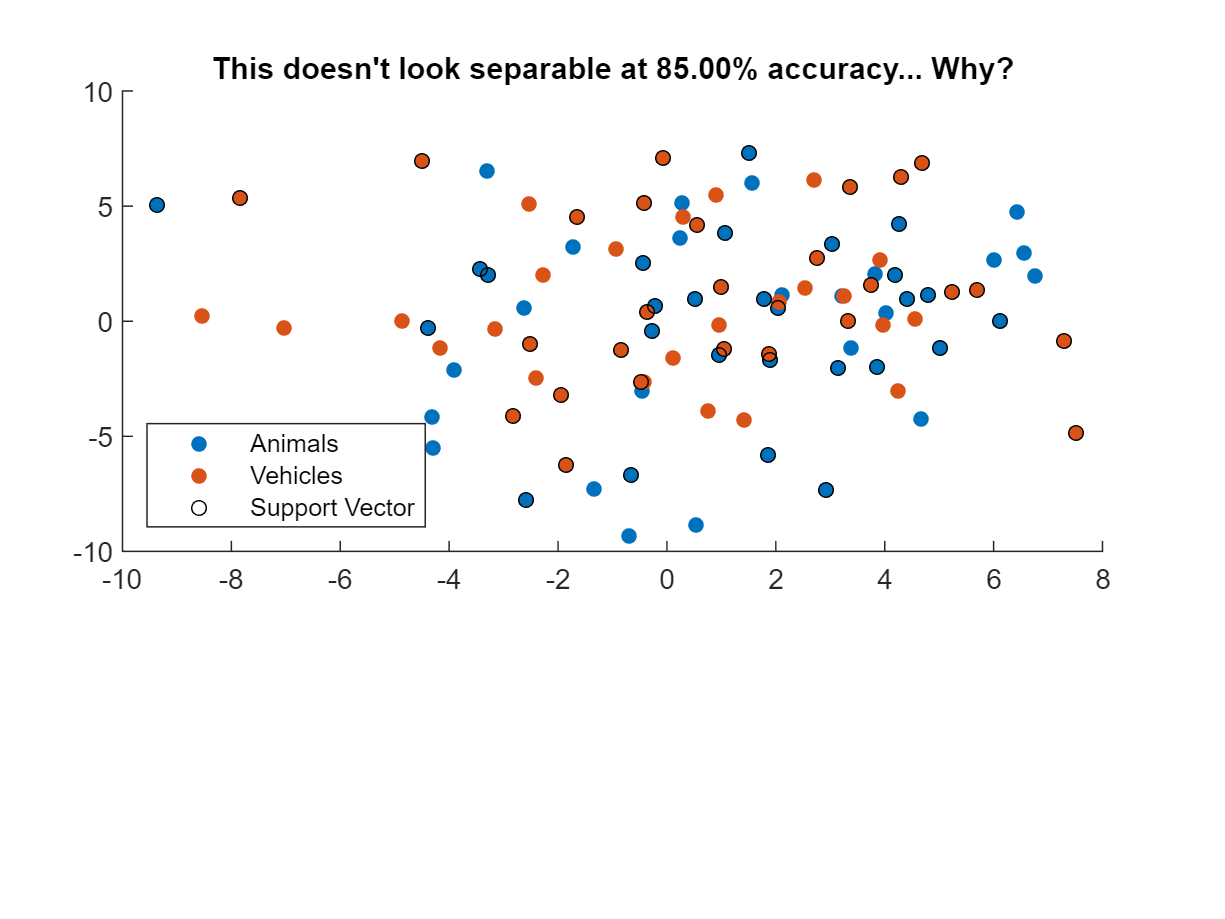
In this case, plotting classifier performance on the training set fails to indicate good performance because we only plotted 2 variables/voxels out of the 100-voxel neural pattern. Now if we repeat MVPA decoding with just two voxels…

1
2
3
4
5
clf = SVC(struct('kernel', 'linear')); % define classifer type
clf.fit(X_train(:, 1:2), y_train); % training
y_pred = clf.predict(X_test(:, 1:2)); % testing
score = accuracy_score(y_test, y_pred); % classification accuracy
fprintf('Accuracy: %.2f%%\n', score*100);

Accuracy: 60.00%

Beyond discrete classification results (“animal” or “vehicle”), we can also get a continuous measure of the “probability” of each datapoint belonging to each class with this simple line of code (which is unfortunately not supported in this sklearn MATLAB toolbox).

1
y_pred_proba = clf.predict_prob(X_test)

Despite all the machine learning hype, we actually do not have to use any machine learning algorithms for decoding analysis. If you remember, the original goal of decoding analysis is to go from (high dimensional) data to (low dimensional) condition, and machine learning is just a tool that sometimes finishes the job neatly. But there are alternatives. Correlation-based MVPA decoding just uses the simple criterion that same-class items should be more correlated (in terms of behavioral ratings, beta estimates, etc.) than different-class items. So we could take the activation pattern of one trial, correlate it with that of both animals and vehicles, and determine the class label of the trial based on whichever correlation coefficient is higher. (This is quite nicely explained in the Coutanche & Thompson-Schill 2013 paper linked at the end.)

We can also use nearest neighbor (left figure) or distance-to-centroid (right) as our criterion with the assumption that same-class items should be closer together than different-class items.

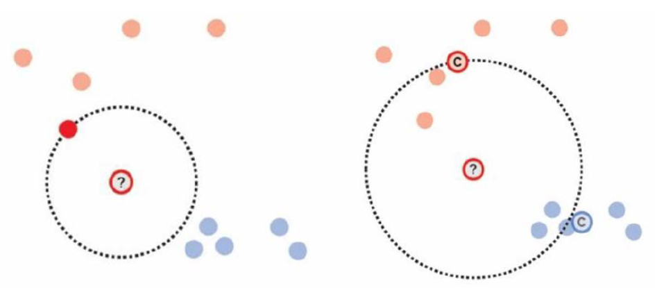
source: Weaverdyck et al. (2020)

But, there are several issues with decoding anlaysis, for many of which I’ll simply refer us to Gessell et al. (2020) linked at the bottom. A more practical issue, though, is that when there are many (say, 10) classes of items, classification results tend to become really poor with the limited amout of fMRI data we usually have for classifier training. (I mean, if you had the money to pay research subjects to be scanned 24/7, why would you even do research?)

Representational similarity analyisis

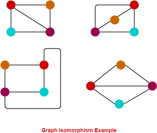
Instead of directly looking at the neural patterns in response to different conditions or stimuli, representational similarity analysis, or RSA, takes a rather indirect route by looking at, well, representational similarity, or second-order isomorphism. Put simply, an isomorphism is a mapping that preserves the structure of the mapped entities. The four graphs below are isomorphic to each other because the relationship beween nodes (all connected except cyan-orange) is preserved in each of them.

source: https://www.gatevidyalay.com/graph-isomorphism/

In the context of cognitive neuroscience and fMRI, the neural activation pattern elicited by something is presumed to be (first-order) isomorphic to the stimulus–the neural representation of an apple and the image of an apple. What we have been doing is compare the neural representations of apples and oranges, with univariate analysis or decoding analysis, and we do so because 1) we believe that apples and oranges are different, 2) such difference should manifest in their respective neural representations because of first-order isomorphism, and 3) it is easy to compare two things.

The downside of first-order isomorphism is that it is not measurable: while we assume there must be a neural representation of apples, we cannot quantify the fidelity of each neural representation in relation to the external stimulus because they are in different formats. This is when second-order isomorphism becomes useful. With a set of stimuli and the corresponding neural patterns, what we can do is first find out the similarity strucutre within the set of stimuli and the similarity structure within the neural patterns, and then compare those two similarity structures; the idea is that similar items will also have similar neural representations.

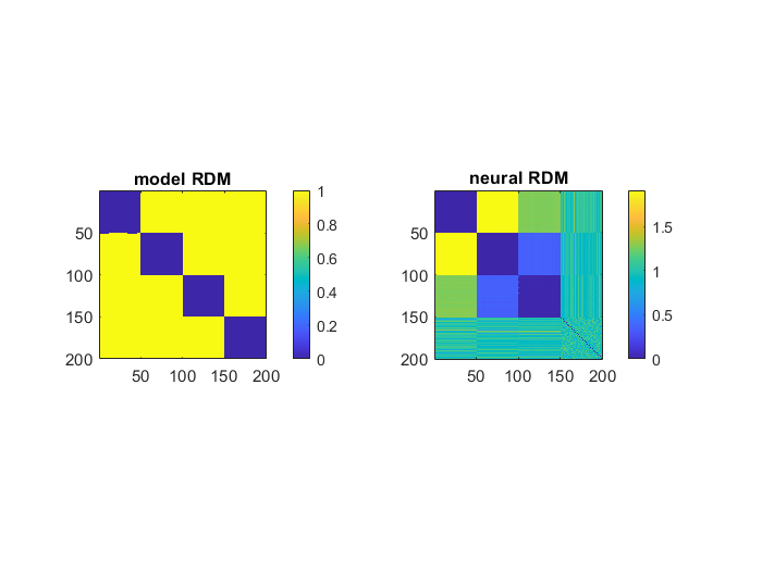
To that end, we will create two representational dissimilarity matrices (RDMs), one for the items and one for the neural patterns. The RDM of neural representations is referred to as the neural RDM, and its computation is depicted in the figure.

source: http://algonauts.csail.mit.edu/img/figure_rdm_v3.png

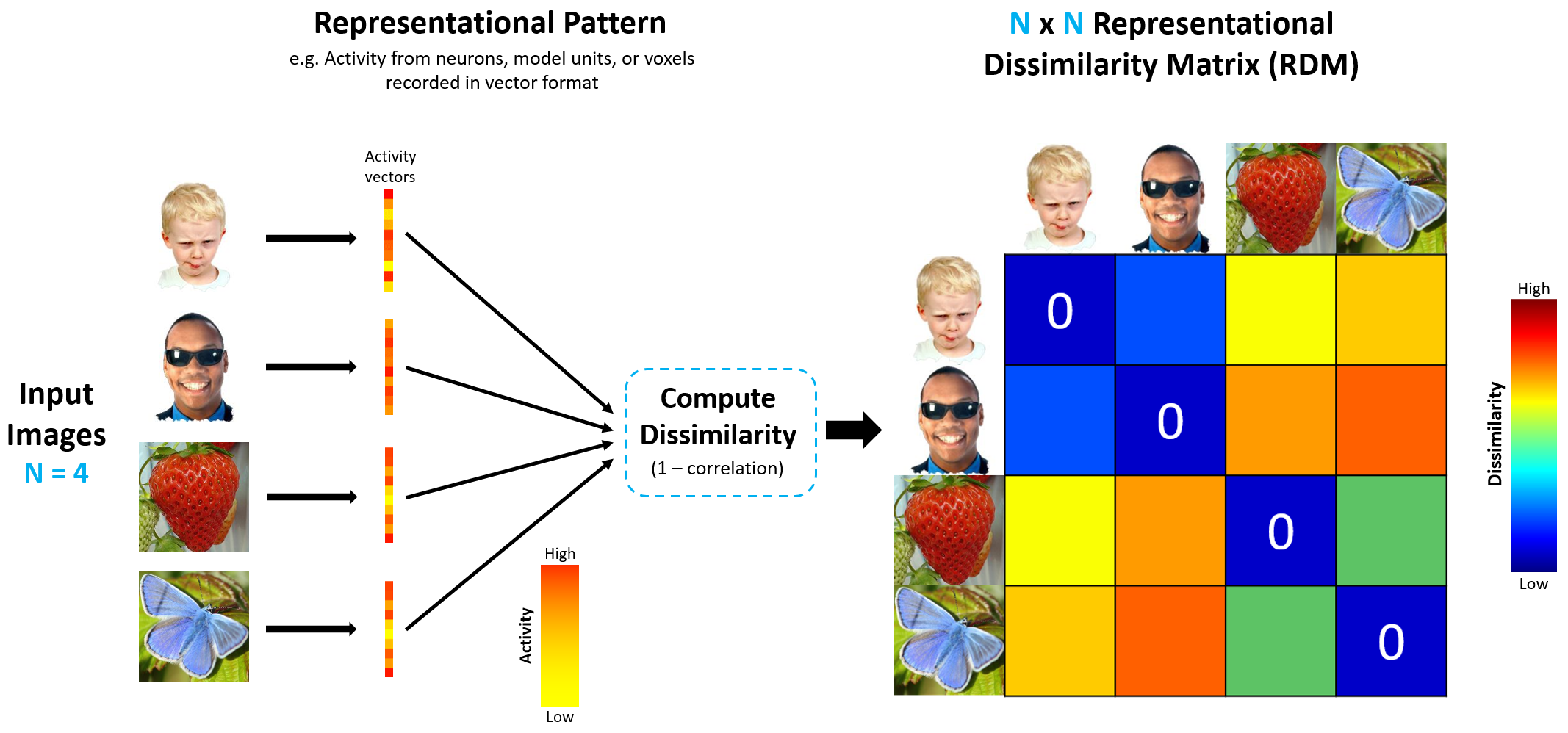
The RDM for items is referred to as the model RDM, because this is our model or hypothesis of how (dis)similar each item is to each other. Using the example in the figure above, we may come up with several different model RDMs:

In all model RDMs, an item is minimally dissimilar (or maximally similar) to itself, so the diagonal entries are always 0. The first model RDM hypothesizes that all faces are minimally dissimilar, all non-faces are minimally dissimilar, and faces are maximally dissimilar to non-faces. The second model RDM hypothesizes that all faces are minimally dissimilar, and any other pair is maximally dissimilar. I leave the most exciting job of interpreting model RDM 3 to the reader.

Unsurprisingly, the model RDM and the neural RDM will be in exactly the same format: both symmetrical matrices of dimension N x N, with N being the number of unique items or trials in the experiment, and this allows us to quantify the second-order isomorphism, usually by computing the correlation between the model RDM and the neural RDM.

1
2
3
4
5
6
7
8
9
10
11
12
13
14
15
16
17
18
19
20
21
22
23
24
25
26
27
28
29
30
31
32
% and yet some more fake data
% this time round we have four types of stimuli, and each appeared times 
beta_pattern_A  = repmat([1; 8; 3], 30, 50) + randn(90,50) * 0.1;
beta_pattern_B  = repmat([9; 0; 3], 30, 50) + randn(90,50) * 0.1;
beta_pattern_C = repmat([5; 4; 3], 30, 50) + randn(90,50) * 0.1;
beta_pattern_D  = repmat([0; 0; 0], 30, 50) + randn(90,50) * 0.1;

% create RDMs
% rows and columns will be in this order: A...A B...B C...C D...D

% all-or-none model RDM
modelRDM = ones(200, 200);
modelRDM(1:50, 1:50) = 0;
modelRDM(51:100, 51:100) = 0;
modelRDM(101:150, 101:150) = 0;
modelRDM(151:200, 151:200) = 0;

% neural RDM
% first concatenate all beta patterns
beta_pattern_A = repmat([1; 8; 3], 30, 50) + randn(90,50) * 0.1;
beta_pattern_B = repmat([9; 0; 3], 30, 50) + randn(90,50) * 0.1;
beta_pattern_C = repmat([5; 4; 3], 30, 50) + randn(90,50) * 0.1;
beta_pattern_D = repmat([0; 0; 0], 30, 50) + randn(90,50) * 0.1;

beta_pattern_all = [beta_pattern_A, beta_pattern_B, beta_pattern_C, beta_pattern_D];
neuralRDM = 1 - corrcoef(beta_pattern_all);

figure;
subplot(1,2,1);
imagesc(modelRDM); colorbar; title('model RDM'); axis('square') 
subplot(1,2,2); 
imagesc(neuralRDM); colorbar; title('neural RDM'); axis('square')

1
2
3
4
5
6
7
8
% quantify second-order isomorphism with second-order correlation between
% model RDM and neural RDM

% only use the lower triangular part without the diagonal entries
% to avoid artificially inflating the correlation coefficient
lowertril = 1:200 < (1:200)';
r = corrcoef(modelRDM(lowertril), neuralRDM(lowertril));
second_order_r = r(1, 2)

second_order_r = 0.6139

There you have it–the second-order isomorphism between a set of external stimuli and each item’s corresponding neural representation, computed as the correlation of correlations–thus a second-order correlation.

Aside (if there’s time)

Classifier- or similarity-hacking

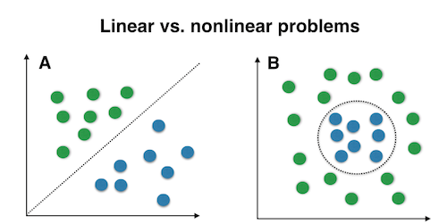
The choice of classifier for decoding analysis and similarity metric for RSA rely on what you hypothesize the underlying data structure would be. Linear and nonlinear classfiers (e.g., SVM with a linear or a RBF kernal) will clearly perform differently for the two problems in the figure. Unfortunately, given the high dimension of fMRI data, we cannot simply plot the data and tell which classifier will perform better.

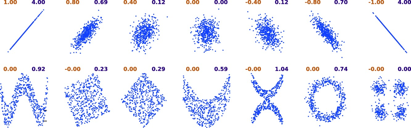
There is also a ton of metrics for the seemingly simple notion of “similarity”. A commonly used on is the Pearson correlation coefficient, which indicates the linear dependence between two random variables. If you have reasons to believe that the relationship will be nonlinear (e.g., y = 1/x), you can either manually transform the data so that the transformed varibles should become linearly related, or use measures like Mutual Information which assumes no particular relationship between two variables–but it is less straightforward to interpret for sure.

What is everyone’s favorite brain region?

This issue is by no means MVPA-specific but essential to almost all fMRI analyses. Searchlight is more exploratory in nature because we usually allow a small cube or sphere to roam around the entire brain, while ROI is more constrained by the anatomy/function of each region based on previous literature. You just gotta pick one.

Or you don’t. Here’s a totally feasible but perhaps worthless idea: we could choose one parcellation of the brain to get, say 400 ROIs, for each subject, and then compute the ROI-level average activation as one would for a univariate activation analysis. Then, instead of using voxels as features as in traditional decoding analysis or RSA, we could first compute the average as one would for a univariate activation analysis, and then conduct decoding analysis or RSA with each ROI as a feature. For what it’s worth, let’s name it multi-region pattern analysis, or MRPA.

To smooth or not to smooth… or to smooth just a little

Spatial smoothing is a preprocessing step that is commonly applied to reduce the noise level in fMRI data. The rationale is that because noise is normally distributed with a mean of 0, by averaging the activation levels of nearby voxels, we will cancel out a fair amount of noise. Univariate activation analysis typically uses (and the default in SPM12 is) full-width at half-maximum (FWHM) at 8 mm.

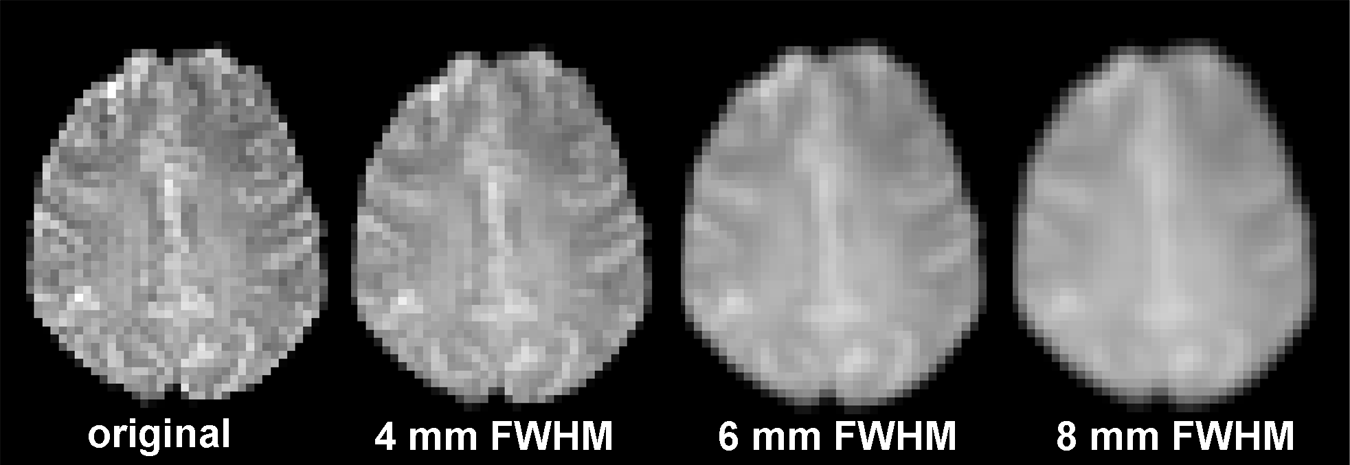
The downside, though, is that we loose the effective spatial resolution in the data. In the extreme case, we can simply average across all brain voxels to get one estimate of the mean activation level of the entire brain–a pretty good estimate because the noise at each voxel will largely cancel out each other, but then a single whole-brain estimate is hardly informative of any specific cognitive process or representation we might be interested in. Ultimately, this issue is a trade-off between the number of unique features and the level of noise you can tolerate, which is possibly different for different cognitive processes or representations.

Why MATLAB?

(This one is for you, Kevin ;)

MATLAB, or MATrix LABoratory, handles matrices quite efficiently, as its name suggests. It works fine for fMRI data analysis, given that fMRI data can be store in matrices of many dimensions (spatial, temporal, cross-subject, etc.). There is also a ton of MATLAB scripts and toolboxes for previous Cabeza lab projects, some of which can be easily adapted to be used for new projects. That said, we can absolutely perform multivariate analysis entirely in other programming languages such as Python–see tutorials on Decoding and RSA from DartBrains.

Resources

• Weaverdyck, M. E., Lieberman, M. D., & Parkinson, C. (2020). Tools of the Trade Multivoxel pattern analysis in fMRI: A practical introduction for social and affective neuroscientists. Social Cognitive and Affective Neuroscience, 15(4), 487–509. https://doi.org/10.1093/scan/nsaa057
• Coutanche, M. N., & Thompson-Schill, S. L. (2013). Informational connectivity: Identifying synchronized discriminability of multi-voxel patterns across the brain. Frontiers in Human Neuroscience, 7. https://doi.org/10.3389/fnhum.2013.00015
• Gessell, B., Geib, B., & De Brigard, F. (2021). Multivariate pattern analysis and the search for neural representations. Synthese. https://doi.org/10.1007/s11229-021-03358-3
• Davis, S. W., Geib, B. R., Wing, E. A., Wang, W.-C., Hovhannisyan, M., Monge, Z. A., & Cabeza, R. (2020). Visual and Semantic Representations Predict Subsequent Memory in Perceptual and Conceptual Memory Tests. Cerebral Cortex. https://doi.org/10.1093/cercor/bhaa269