General Machine Learning

Here’s another lil machine learning tutorial thing - this time instead of neural networks, we’ll be taking a step back to look at machine learning in general! For more specific background on things like linear algebra, please go back and look at Pranjal’s linear algebra presentation, it was a banger and I highly recommend it.

Before we dive in, here’s a quick overview of what we’ll be talking about today.

• What is machine learning (ML)?
• Different types of ML
  • Supervised
  • Unsupervised
• Different subtypes typically used in Science
  • Prediction/classification
  • Generative Modeling
• Good practices in Machine Learning
  • Generalization/overfitting
  • Data Normalization
  • Regularization

What is Machine Learning?

You may have come across machine learning in newspapers or magazines or the internet or really anywhere because it truly seems to be everywhere these days. It’s kind of a buzzword that has been applied to so many things that it doesn’t mean that much anymore. However, generally, it’s exactly what it sounds like: trying to get machines to learn something. This has been applied successfully and unsuccesfully. This is a tricky problem due to how vague it is, so generally it helps if we split it up in to better-defined subclasses.

Types of machine learning

When thinking about ML, we can pretty cleanly split it into two types: supervised learning and unsupervised learning. These two types differ mainly in the type of information we give our ML models and what we expect them to do.

Supervised learning

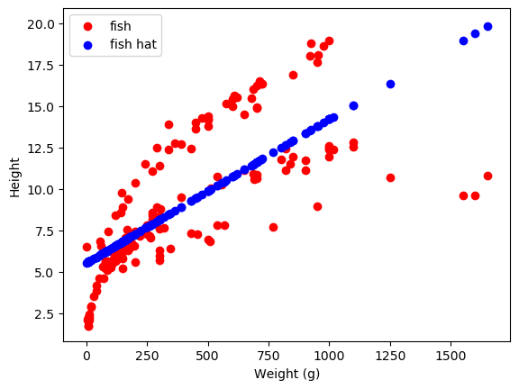
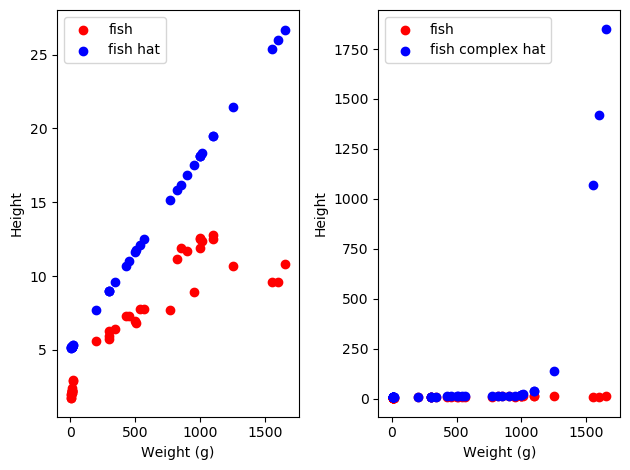
One of the most common types of ML is supervised learning. The name comes from the fact that we as researchers are telling the model exactly what to learn, supervising its learning. In this type of ML, we give our models data (x) and labels (y). The model learns the relationship between the data and the labels and can be used to predict labels from new data new data. One type of supervised learning, which we have tutorials on, is linear regression. In linear regression, we’re generally trying to take a set of features of a dataset and predict outcomes from those features. As a quick little example, let’s use the FISH dataset! This has: fish. Our quick little example will be predicting the height of the fish from the weight. This method will fit a line to our data, here our y is ‘height’ and our x is ‘weight’. The formula we are fitting is \(\begin{equation*} height = w * weight + b \end{equation*}\) where \(w\) is a slope indicating the relationship between weight and height, and \(b\) is a baseline offset.

1
2
3
4
5
6
7
8
9
10
11
12
13
14
15
16
17
18
19
20
21
22
23
import pandas as pd
from sklearn.linear_model import LinearRegression as LR
import matplotlib.pyplot as plt
import numpy as np

fish = pd.read_csv('fish.csv').dropna()

x = fish['Weight'].to_numpy()
y = fish['Height'].to_numpy()

fish_model = LR().fit(x[:,np.newaxis],y)

yhat = fish_model.predict(x[:,np.newaxis])


ax = plt.gca()

data = ax.scatter(x,y,c='r')
predictions = ax.scatter(x,yhat,c='b')
ax.set_xlabel('Weight (g)')
ax.set_ylabel('Height')
plt.legend([data,predictions],['fish','fish hat'])
plt.show()

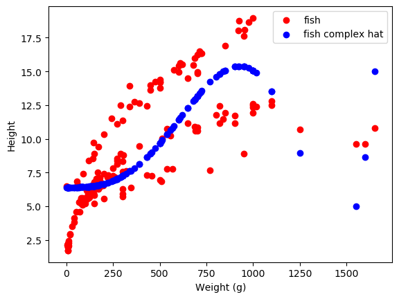
as a ~ sneak peek ~ for future sections, we can also make our model more complicated to fit our data better

1
2
3
4
5
6
7
8
9
10
11
12
13
14
15
16
17
18
19
20
21
#x2 = x**2
x3 = x**3
#x4 = x**4
x5 = x**5
x7 = x**7
logfish = np.log(x+1e-3)
x_complex = np.stack([x,x3,x5,x7,logfish],axis=1)

fish_model_complex = LR().fit(x_complex,y)

yhat_complex = fish_model_complex.predict(x_complex)


ax = plt.gca()

data = ax.scatter(x,y,c='r')
predictions = ax.scatter(x,yhat_complex,c='b')
ax.set_xlabel('Weight (g)')
ax.set_ylabel('Height')
plt.legend([data,predictions],['fish','fish complex hat'])
plt.show()

Yay! that does fine I guess. Time to move onto unsupervised learning!!

Unsupervised learning

In unsupervised learning, we just give our model data and we leave and say “figure it out!” That’s why it’s unsupervised - the model learns whatever it thinks is useful. Popular methods of this include things like K-Means clustering and agglomerative clustering. These can be really nice when you don’t have labels, or during exploratory data analysis they can be good for understanding where there is structure in our data. It looks like there are three (3) clusters in our height and weight data, so let’s see how different types of unsupervised learning do at representing our data.

We’ll try out K-Means and hierarchical agglomerative clustering. K-Means selects cluster centers. Then it assigns all our data points to their closest center. Next, it updates the cluster centers to be the center of mass of their labelled data. It continues to do this until it does well.

Hierarchical agglomerative clustering works a little bit differently. It starts off with each point as its own individual cluster. Next it merges the two closest clusters. It keeps doing this until it reaches our desired number of clusters.

Let’s try clustering by everything and plotting along height and weight!

1
2
3
4
5
6
7
8
9
10
11
12
13
14
15
16
17
18
19
20
21
22
23
24
25
26
27
28
29
30
31
32
33
34
from sklearn.cluster import AgglomerativeClustering as AC
from sklearn.cluster import KMeans as KM

#print(fish.columns)
#data = fish.drop(['Species'],axis=1).to_numpy()#[['Height','Length2']].to_numpy()
xy = fish[['Weight','Height']].to_numpy()
#xy = np.stack([x,y],axis=1)

AC_fish = AC(n_clusters=3)

KM_fish = KM(n_clusters=3)

xy_labs_AC = AC_fish.fit_predict(xy)
xy_labs_KM = KM_fish.fit_predict(xy)

fig, (ax1,ax2) = plt.subplots(1,2)

l1 = ax1.scatter(xy[xy_labs_AC == 0,0],xy[xy_labs_AC == 0,1],c='r')
l2 = ax1.scatter(xy[xy_labs_AC == 1,0],xy[xy_labs_AC == 1,1],c='g')
l3 = ax1.scatter(xy[xy_labs_AC == 2,0],xy[xy_labs_AC == 2,1],c='b')
ax1.set_xlabel('Weight (g)')
ax1.set_ylabel('Height')
ax1.legend([l1,l2,l3],['Cluster 1','Cluster 2', 'Cluster 3'])
ax1.set_title('Cluster identities by Agglomerative Clustering')

l1 = ax2.scatter(xy[xy_labs_KM == 0,0],xy[xy_labs_KM == 0,1],c='r')
l2 = ax2.scatter(xy[xy_labs_KM == 1,0],xy[xy_labs_KM == 1,1],c='g')
l3 = ax2.scatter(xy[xy_labs_KM == 2,0],xy[xy_labs_KM == 2,1],c='b')
ax2.set_xlabel('Weight (g)')
ax2.set_ylabel('Height')
ax2.legend([l1,l2,l3],['Cluster 1','Cluster 2', 'Cluster 3'])
ax2.set_title('Cluster identities by K-Means')
fig.tight_layout()
plt.show()

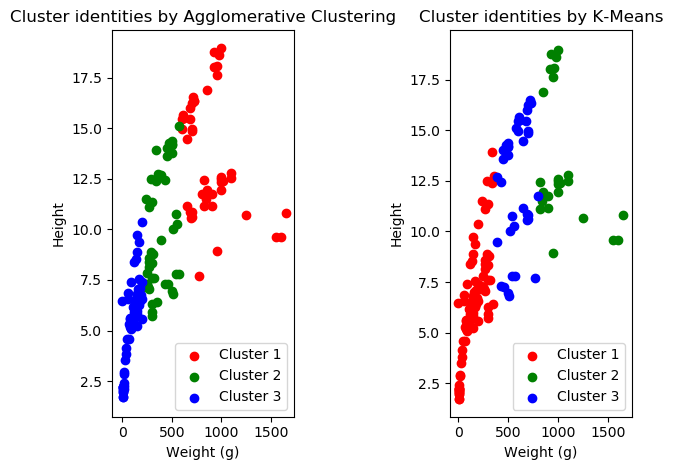
Wow! Look at that! They don’t do well! However, they both do slightly different things. Also, cluster identity changes based on how we initialize our machine learning algorithm. If you run this code multiple times, you’ll get different results! Anyway, this is just a quick overview of different types of ML so we’re not going to go too much more in-depth about this! If you want to know more about clustering, peer pressure me into doing another one of these methods meetings.

ML Subtypes typically used in science

While the supervised/unsupervised dichotomy is kind of nice when thinking about things in a strictly machine-learning sense, it can also be important to split up ML in other ways! In Science, I’ve typically seen things split into classification/prediction and generative modeling as the two main subtypes. (note: the real name that classification/prediction models fall under is discriminative models, but since we mainly use them for classification/prediction in Science that’s what I’m calling them here)

Classification/prediction

contains everything that we saw previously, both supervised and unsupervised, as well as fun things like logistic regression, which we should have a tutorial on if we have not already (but which is also briefly mentioned here).

On the other hand, we have

Generative modeling

I hope you don’t mind that I switch how I spell modelling when I write. It’s because I can’t make up my mind. Generative modeling imposes certain assumptions on how the data were ~ generated ~. Broadly speaking, this class of models deals with the assumption that in any given dataset, there are only a few factors that actually control the variance in the data. These are known as latent factors. You can think of this through the (more) simple example of dogs. If you see a dog, you know it belongs to the general category of dogs, but it is distinct from all others in some ways. However, even though the dog takes up a lot of visual space, the ways in which it is distinct from others is limited. It can differ in terms of size, snout length, fur color, ear size, etc. These factors which I just listed would be latent, since they actually account for the variance in what dogs look like, rather than considering every single hair on its body to be different from every other dog’s. The goal of generative modeling is: given a dataset, uncover the latent factors.

This is done typically through a few types of models, I use VARIATIONAL AUTOENCODERS in my work, but we can also consider things like hidden markov models to be generative models. They are BEYOND THE SCOPE of this notebook so again: peer pressure me

Good Practices in Machine Learning

Finally, we have arrived at the last stop on our magical machine learning (m)adventure. Good practices in machine learning. Although we can get some really powerful and very cool models with machine learning that can do a GREAT job of predicting our outcomes of interest - we have to be careful to make sure that they learn something that is actually useful. We want our model to be powerful enough to fit our data, but too weak to fit to noise in our data. Our data do not follow a strict one-to-one relationship with our outcomes ever; they always follow a general, average relationship plus some added noise. Therefore we can consider our data to be distributed according do some overall universal data distribution:

\(\begin{equation*} x \sim P(\mathcal{D}) \end{equation*}\) Where \( \mathcal{D} \) is every single possible data point, \( P(\mathcal{D}) \) is the probability distribution over those data points, and \(x\) is our actual realization of our data. Under this framework, we want our model to learn based on the full population of data, not just our realization of it. The ability of our model to learn the full data structure is known as generalization. If our model overfits to our noisy realization of the data, that’s known as overfitting. To make sure we don’t overfit to our data, we generally split our data into a train set and a test set. When learning, the model only sees our train set and then we test it on the test set. This way we kind of simulate all that extra mystery population that we don’t have access to, by witholding part of the actual data that we do have.

Let’s consider the case where we have our fish and want to make a linear model, and let’s consider our complex fish and our simple fish. We might get really unlucky and just get a bad split of data, in which case we might see something like the following:

1
2
3
4
5
6
7
8
9
10
11
12
13
14
15
16
from sklearn.model_selection import train_test_split as tts


n_train = int(len(x)*0.75)

X_train = x[0:n_train][:,np.newaxis]
X_test = x[n_train::][:,np.newaxis]
y_train = y[0:n_train]
y_test = y[n_train::]

ax = plt.gca()

ax.scatter(X_train,y_train,c='r')
ax.scatter(X_test,y_test,c='b')

plt.show()

In this case, we get a bad split of our data, and are missing about half of our distribution! Our train set is in red, our test set is in blue. Let’s see how our models do on this:

1
2
3
4
5
6
7
8
9
10
11
12
13
14
15
16
17
18
19
20
21
22
23
24
25
26
27
28
29
30
31
32
33
34
35
36
37
38
39
40
41
42
43
44
45
46
47
48
#x2 = x**2
x3tr = X_train**3
#x4 = x**4
x5tr = X_train**5
x7tr = X_train**7
logfishtr = np.log(X_train+1e-3)

x3te = X_test**3
#x4 = x**4
x5te = X_test**5
x7te = X_test**7
logfishte = np.log(X_test+1e-3)

x_complex_train = np.hstack([X_train,x3tr,x5tr,x7tr,logfishtr])
x_complex_test = np.hstack([X_test,x3te,x5te,x7te,logfishte])

fish_model_simple = LR().fit(X_train,y_train)
fish_model_complex = LR().fit(x_complex_train,y_train)

yhat_train_simple = fish_model_simple.predict(X_train)
yhat_train_complex = fish_model_complex.predict(x_complex_train)
yhat_test_simple = fish_model_simple.predict(X_test)
yhat_test_complex = fish_model_complex.predict(x_complex_test)

train_acc_simple = np.mean((yhat_train_simple - y_train)**2)
train_acc_complex = np.mean((yhat_train_complex - y_train)**2)
test_acc_simple = np.mean((yhat_test_simple - y_test)**2)
test_acc_complex = np.mean((yhat_test_complex - y_test)**2)

print('Train Error Simple: {}, Train Error Complex: {}'.format(train_acc_simple,train_acc_complex))
print('Test Error Simple: {}, Test Error Complex: {}'.format(test_acc_simple,test_acc_complex))

fig,(ax1,ax2) = plt.subplots(1,2)

data = ax1.scatter(X_test,y_test,c='r')
predictions = ax1.scatter(X_test,yhat_test_simple,c='b')
ax1.set_xlabel('Weight (g)')
ax1.set_ylabel('Height')
ax1.legend([data,predictions],['fish','fish hat'])

data = ax2.scatter(X_test,y_test,c='r')
predictions = ax2.scatter(X_test,yhat_test_complex,c='b')
ax2.set_xlabel('Weight (g)')
ax2.set_ylabel('Height')
ax2.legend([data,predictions],['fish','fish complex hat'])

fig.tight_layout()
plt.show()

1
2
Train Error Simple: 3.828587659678313, Train Error Complex: 4.075698918694715
Test Error Simple: 39.83401397133755, Test Error Complex: 163084.93536380908

As we can see, both of our models do pretty well on the train set. However, on our test data, our complex model does way worse than our simple model! This is because our complex model was allowed to fit more fully to the noise in the data, resulting in overall worse model performance on the data distribution as a whole. We can help our models out with this by splitting our data into training and test sets always, and using the performance on the test set to see how well our model is doing. That way we can be sure we don’t overfit to our data specifically!

Normalization

One other tip and trick that is good to follow is that of data normalization. Sometimes, our data might be on entirely different scales from one another! In our dataset, we can see this with the difference between height and weight. Weight is in grams while height is in cm, and there are completely different possible ranges for each feature. Therefore it can be good to normalize each feature, generally so that each is mean centered with a standard deviation of 1, so that no feature is viewed as more important than any other simply due to its magnitude. Some other ways are: just mean centering the data, and scaling it to range from zero to one. these look like this:

1
2
3
4
5
6
7
8
9
10
11
12
13
14
15
16
17
18
19
20
21
22
23
24
25
26
x_centered_scaled = (x - np.mean(x))/np.std(x)

x_centered = x - np.mean(x)

x_scaled = x/np.max(x)

fig,(ax1,ax2,ax3) = plt.subplots(1,3)

data = ax1.scatter(x_centered_scaled,y,c='r')
#predictions = ax1.scatter(centered_x,y,c='b')
ax1.set_xlabel('Weight')
ax1.set_ylabel('Height')
#ax1.legend([data,predictions],['fish','fish hat'])

data = ax2.scatter(x_centered,y,c='r')
#predictions = ax2.scatter(X_test,yhat_test_complex,c='b')
ax2.set_xlabel('Weight')
ax2.set_ylabel('Height')
#ax2.legend([data,predictions],['fish','fish complex hat'])

data = ax3.scatter(x_scaled,y,c='r')
#predictions = ax2.scatter(X_test,yhat_test_complex,c='b')
ax3.set_xlabel('Weight')
ax3.set_ylabel('Height')
fig.tight_layout()
plt.show()

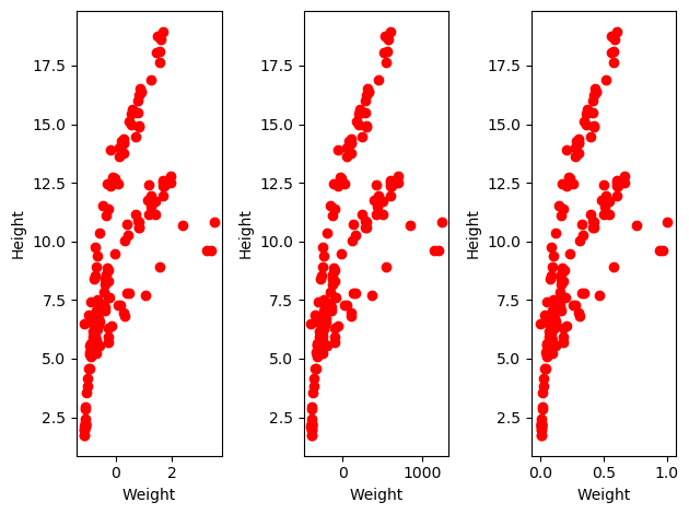
So as you can see from the above, with normalization the overall TRENDS in the data stay the same, but the numbers lay in a much tighter range (except in the centering case), making it (potentially) easier for our models to understand these trends. Does this do anything in practice?

1
2
3
4
5
6
7
8
9
10
11
12
13
14
15
16
17
18
19
20
21
22
23
24
25
26
27
28
29
30
31
32
33
xy_labs_cs = AC_fish.fit_predict(np.stack([x_centered_scaled,y],axis=1))
xy_labs_c = AC_fish.fit_predict(np.stack([x_centered,y],axis=1))
xy_labs_s = AC_fish.fit_predict(np.stack([x_scaled,y],axis=1))


fig, (ax1,ax2,ax3) = plt.subplots(1,3)

l1 = ax1.scatter(x_centered_scaled[xy_labs_cs == 0],y[xy_labs_cs == 0],c='r')
l2 = ax1.scatter(x_centered_scaled[xy_labs_cs == 1],y[xy_labs_cs == 1],c='g')
l3 = ax1.scatter(x_centered_scaled[xy_labs_cs == 2],y[xy_labs_cs == 2],c='b')
ax1.set_xlabel('Weight')
ax1.set_ylabel('Height')
ax1.legend([l1,l2,l3],['Cluster 1','Cluster 2', 'Cluster 3'])
#ax1.set_title('Cluster identities by Agglomerative Clustering')

l1 = ax2.scatter(x_centered[xy_labs_c == 0],y[xy_labs_c == 0],c='r')
l2 = ax2.scatter(x_centered[xy_labs_c == 1],y[xy_labs_c == 1],c='g')
l3 = ax2.scatter(x_centered[xy_labs_c == 2],y[xy_labs_c == 2],c='b')
ax2.set_xlabel('Weight')
ax2.set_ylabel('Height')
#ax1.legend([l1,l2,l3],['Cluster 1','Cluster 2', 'Cluster 3'])
#ax1.set_title('Cluster identities by Agglomerative Clustering')

l1 = ax3.scatter(x_scaled[xy_labs_s == 0],y[xy_labs_s == 0],c='r')
l2 = ax3.scatter(x_scaled[xy_labs_s == 1],y[xy_labs_s == 1],c='g')
l3 = ax3.scatter(x_scaled[xy_labs_s == 2],y[xy_labs_s == 2],c='b')
ax3.set_xlabel('Weight')
ax3.set_ylabel('Height')
#ax1.legend([l1,l2,l3],['Cluster 1','Cluster 2', 'Cluster 3'])
#ax1.set_title('Cluster identities by Agglomerative Clustering')

fig.tight_layout()
plt.show()

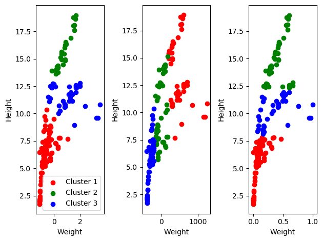
Why yes it does! that’s why I’m telling you about it. I wish I’d chosen a better dataset for this, but oh well. Regardless, the clusters depend on the data and we get different outcomes based on how we scale our data.

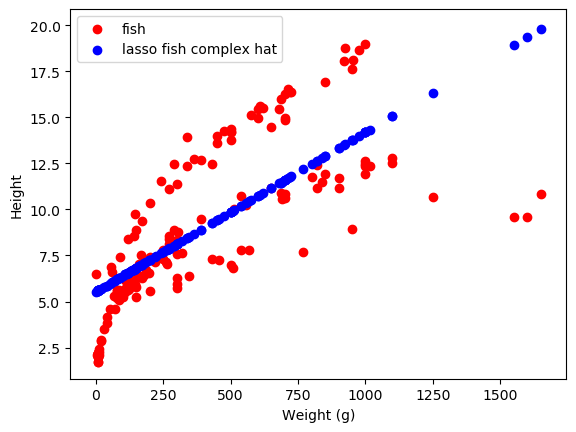
Regularization

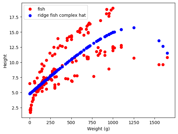
Finally, we can regularize our models to make sure they don’t overfit. Regularization adds an extra term that our models have to satisfy, basically constraining the size of the weights in the model. This can help in several ways. The first typical way is through ridge regression, or L2 normalization on linear regression. L2 normalization penalizes the squared size of the weights. This prevents any weight on any feature from getting TOO large, meaning that no feature can seriously outweigh any other unless it is really important.

There is also Lasso Regression, or L1 normalization on linear regression. This penalizes the size of the weights. This actually ends up encouraging sparsity in the weights - this regularization tends to force most of the weights towards zero, prioritizing just the few most important ones.

1
2
3
4
5
6
7
8
9
10
11
12
13
14
15
16
17
18
19
20
21
22
23
24
25
26
27
28
29
30
31
32
33
34
35
36
37
from sklearn.linear_model import Ridge, Lasso

#x2 = x**2
x3 = x_scaled**3
#x4 = x**4
x5 = x_scaled**5
x7 = x_scaled**7
#logfish = np.log(x+1e-3)
x_complex_s = np.stack([x,x3,x5,x7],axis=1)

fish_model_r= Ridge(alpha=2).fit(x_complex_s,y)
fish_model_l= Lasso(alpha=2).fit(x_complex_s,y)

yhat_r = fish_model_r.predict(x_complex_s)
yhat_l = fish_model_l.predict(x_complex_s)


ax = plt.gca()

data = ax.scatter(x,y,c='r')
predictions = ax.scatter(x,yhat_r,c='b')
ax.set_xlabel('Weight (g)')
ax.set_ylabel('Height')
plt.legend([data,predictions],['fish','ridge fish complex hat'])
plt.show()

ax = plt.gca()

data = ax.scatter(x,y,c='r')
predictions = ax.scatter(x,yhat_l,c='b')
ax.set_xlabel('Weight (g)')
ax.set_ylabel('Height')
plt.legend([data,predictions],['fish','lasso fish complex hat'])
plt.show()

print('Ridge coefficients: ',fish_model_r.coef_)
print('Lasso coefficients: ',fish_model_l.coef_)

1
2
Ridge coefficients:  [ 0.01168738 -4.90564603 -4.18956067 -3.44761545]
Lasso coefficients:  [ 0.00865715 -0.         -0.         -0.        ]

As we can see, these do different things! The weights learned by lasso are mainly zero, while those learned by Ridge are (relatively) small-ish. The \(\alpha\) parameter changes how much weight there is on this regularization term - larger alpha means that the size of the weights will be more heavily penalized. There are more methods of regularization, but these are the main ones I’ve run into in Science!

Anyway hope you enjoyed send me questions if you want