-
Why MATLAB?
-
Getting started
-
Data types
3.1 Numeric types
3.2 Characters and Strings
3.3 Tables
3.4 Cell Arrays
3.5 Structures
-
Regression
-
Conclusion
1. Why MATLAB?
MATLAB is a proprietary programming language and computing enviorment developed by MathWorks. It is specifically desinged for engineers and scientists who work with data matrices of large sizes. Some of its advantages over other options (e.g., R, Python) include:
- having a graphical user interface (GUI)
- (relatively) easy-to-understand data types
- comprehensive tried-and-tested built-in functions
- various toolboxes for brain research and beyond
Here are some famous/useful packages that you’ll likely come across in research:
| Name |
Description |
| SPM |
one of the most popular packages for preprocessing and analyzing neuroimaging data, besides FSL and AFNI |
| CONN |
MATLAB- and SPM-based interactive toolbox for analyzing brain connectivity |
| EEGLAB |
interactive toolbox for processing EEG, MEG, and other electrophysiological data |
| FieldTrip |
non-interactive toolbox for processing MEG, EEG, and iEEG data |
| PsychToolbox |
toolbox for controling visual and auditory stimulus presentation |
And here are some previous DIBS Methods Meeting posts that included some MATLAB code snippets:
Hopefully this is just enough to convince you of the usefulness of MATLAB!
2. Getting started
If you haven’t installed MATLAB or want to familiarize yourself with the GUI, please refer to my earlier post on MATLAB basics. Alternatively, you can try out the online version here without the hassle of installation: https://matlab.mathworks.com/.
Also feel free to download this MATLAB livescript to follow along.
3. Data types
Data types and basic operations in MATLAB were covered in a bit more depths in my earlier post, but we are going to to quickly review some important things here because they will come up later as we talk about regressions in MATLAB.
Numeric types
There are several numeric types in MATLAB:
- double Double-precision arrays (64-bit) <– MATLAB default
- single Single-precision arrays (32-bit)
- int8 8-bit signed integer arrays
- uint8 8-bit unsigned integer arrays
1
| class(1) % use the function `class` to check data types
|
As mentioned before, one of the advantages of MATLAB is it’s efficient handling of matrices or arrays, which we can easily assemble as below
1
2
3
4
5
| % use space or comma to separate columns
% use semicolon to separate rows
% use square brackets [ ] to put things together
a = [1 2, NaN;
.5 Inf nan]
|
This code defines a 2 x 3 (double) array:
1
2
3
| a = 2x3
1.0000 2.0000 NaN
0.5000 Inf NaN
|
Characters and Strings
Both single and double quotes can be used for text data. While they are really interchangeable in Python and R, they have very difference functions in MATLAB. Single quotes ' ' create a sequence of characters, whereas double quotes " " create a complete piece string.
1
2
3
4
5
6
| %%% use single quotes for characters
char1 = 'a';
char2 = 'abc';
%%% use double quotes for strings
str1 = "a";
str2 = "abc";
|
You can see the difference in the length of 'abc' and "abc".
Similar to numbers, text data can be assembled together into arrays, though it’s more complicated with the distinction between characters and strings.
First, if we want to concatenate text,
1
| [char1 char2] % correctly concatenated character array
|
1
| str1 + str2 % correctly concatenated strings
|
However, we cannot use addition for two characters
1
| char1 + char2 % data type converted to numeric for addition
|
1
2
| ans = 1x3
194 195 196
|
Neither can we use [ ] for concatenation of strings, as it will give use an array.
1
| [char1 str2] % character coerced to string
|
1
2
| ans = 1x2 string
"a" "abc"
|
Tables
Tables in MATLAB are similar to data frames in Python (Pandas) and R. They are really useful for data organization, and we will use them for regression analyses later.
Let’s define an example table in MATLAB with 2 rows and 2 columns.
1
2
3
4
| T = table;
T.col1 = [1; 2];
T.col2 = ["hello"; "world"];
T
|
| |
col1 |
col2 |
| 1 |
1 |
“hello” |
| 2 |
2 |
“world” |
When we add new data into an existing table, the dimensions must match.
1
2
3
| % dimensions must match
T.col3 = repmat(3, height(T), 1);
try T.col4 = 4; catch err; disp(err); end
|
1
2
3
4
5
6
7
| MException with properties:
identifier: 'MATLAB:table:RowDimensionMismatch'
message: 'To assign to or create a variable in a table, the number of rows must match the height of the table.'
cause: {}
stack: [2x1 struct]
Correction: []
|
Another thing that table enforces is data type. All entries in the same column must have the same data type, e.g., string.
1
2
3
| % data type must be consistent within each row
T.col2(2) = 1;
T % see how 1 is coerced into "1"
|
| |
col1 |
col2 |
col3 |
| 1 |
1 |
“hello” |
3 |
| 2 |
2 |
“1” |
3 |
Cell
Cell is another container data type that can be used to flexibly store data. It is flexible because there is no restriction on the data type that is stored in each cell. Let’s define an example cell array with 3 rows and 2 columns.
1
2
| % use curly brackets to put together things of different sizes and types
C = {42, "abcd"; table(nan), [1 2 3]; Inf, {}}
|
| |
1 |
2 |
| 1 |
42 |
“abcd” |
| 2 |
1x1 table |
[1,2,3] |
| 3 |
Inf |
0x0 cell |
There are two ways to index a cell array, using ( ) or { }.
1
| C(2) % paratheses indexing retrieves the cell
|
1
| C{2} % curly braces indexing retrieves the cell *content*
|
As an aside, arrays are effcient, but we have to make sure that we access them in the correct order.
1
2
3
| % double arrays are indexed with parentheses
a = [11 12 13; 21 23 24]; % 2 x 3 double array
a
|
1
2
3
| a = 2x3
11 12 13
21 23 24
|
1
| a(1, 2) % row 1, column 2
|
1
| a(1:end, 2) % all rows, column 2
|
1
| a(2, :) % row 2, all columns
|
Here’s something that may seem odd – we can actually access the entries with just one index.
Let’s look at how MATLAB interally stores the entries in this array.
1
2
3
4
5
6
7
| ans = 6x1
11
21
12
23
13
24
|
In Python and R, array data is stored row-wise. In contrast, MATLAB arrays are stored column-wise, even though they are easily defined row-wise.
┑( ̄Д  ̄)┍
Structures
This is probably the most versatile data type in MATLAB, and many complex functions and toolboxes make extensive uses of this data type. A structure can contain multiple fields, each of which can be of whatever data type.
1
2
3
4
5
6
7
8
| % group data using fields
% each field can be of any data type, including structures
S = struct;
S.field1_struct = struct;
S.field2_cell = C;
S.field3_table = T;
S.field4_char = char1;
S
|
1
2
3
4
5
| S =
field1_struct: [1x1 struct]
field2_cell: {3x2 cell}
field3_table: [2x3 table]
field4_char: 'a'
|
After reviewing all these data types, we should be ready to fit some regression models in MATLAB!
4. Regression
Through the official Statistics and Machine Learning Toolbox, we have access to several built-in MATLAB functions for regression.
First, let’s load some example data. We are going to use an open dataset on Kaggle on life expectancy. The original data came from the World Health Organization (WHO), who has been keeping track of the life expectancy and many other health factors of all countries. The final dataset consists of 20 predictor variables and 2938 rows, containing information for 193 countries between 2000 and 2015. Download this dataset here.
1
2
3
| data_table = readtable("2024-03-01-matlab-regression-Life-Expectancy.csv", ...
"VariableNamingRule", "preserve"); % preserve white space in column names for readability
head(data_table);
|
1
2
3
4
5
6
7
8
9
10
11
| Country Year Status Life expectancy Adult Mortality infant deaths Alcohol percentage expenditure Hepatitis B Measles BMI under-five deaths Polio Total expenditure Diphtheria HIV/AIDS GDP Population thinness 1-19 years thinness 5-9 years Income composition of resources Schooling
_______________ ____ ______________ _______________ _______________ _____________ _______ ______________________ ___________ _______ ____ _________________ _____ _________________ __________ ________ ______ __________ ____________________ __________________ _______________________________ _________
{'Afghanistan'} 2015 {'Developing'} 65 263 62 0.01 71.28 65 1154 19.1 83 6 8.16 65 0.1 584.26 3.3736e+07 17.2 17.3 0.479 10.1
{'Afghanistan'} 2014 {'Developing'} 59.9 271 64 0.01 73.524 62 492 18.6 86 58 8.18 62 0.1 612.7 3.2758e+05 17.5 17.5 0.476 10
{'Afghanistan'} 2013 {'Developing'} 59.9 268 66 0.01 73.219 64 430 18.1 89 62 8.13 64 0.1 631.74 3.1732e+07 17.7 17.7 0.47 9.9
{'Afghanistan'} 2012 {'Developing'} 59.5 272 69 0.01 78.184 67 2787 17.6 93 67 8.52 67 0.1 669.96 3.697e+06 17.9 18 0.463 9.8
{'Afghanistan'} 2011 {'Developing'} 59.2 275 71 0.01 7.0971 68 3013 17.2 97 68 7.87 68 0.1 63.537 2.9786e+06 18.2 18.2 0.454 9.5
{'Afghanistan'} 2010 {'Developing'} 58.8 279 74 0.01 79.679 66 1989 16.7 102 66 9.2 66 0.1 553.33 2.8832e+06 18.4 18.4 0.448 9.2
{'Afghanistan'} 2009 {'Developing'} 58.6 281 77 0.01 56.762 63 2861 16.2 106 63 9.42 63 0.1 445.89 2.8433e+05 18.6 18.7 0.434 8.9
{'Afghanistan'} 2008 {'Developing'} 58.1 287 80 0.03 25.874 64 1599 15.7 110 64 8.33 64 0.1 373.36 2.7294e+06 18.8 18.9 0.433 8.7
|
Let’s validate the information in the description above.
1
2
3
4
5
6
7
| fprintf( ...
"Number of rows = %d \n" + ...
"Number of years = %d \n" + ...
"Number of countries = %d \n", ...
height(data_table), ...
length(unique(data_table.Year)), ...
length(unique(data_table.Country)));
|
1
2
3
| Number of rows = 2938
Number of years = 16
Number of countries = 193
|
For simplicity, we are going to focus on the most recent complete sample (year 2014) and on the following variables:
- Life expectancy (in years)
- Status: “Developed”, “Developing”
- Total expenditure: General government expenditure on health as a percentage of total government expenditure (%)
1
2
| data_2014 = data_table(data_table.Year==2014, ["Country" "Status" "Total expenditure" "Life expectancy"]);
head(data_2014);
|
1
2
3
4
5
6
7
8
9
10
11
| Country Status Total expenditure Life expectancy
_______________________ ______________ _________________ _______________
{'Afghanistan' } {'Developing'} 8.18 59.9
{'Albania' } {'Developing'} 5.88 77.5
{'Algeria' } {'Developing'} 7.21 75.4
{'Angola' } {'Developing'} 3.31 51.7
{'Antigua and Barbuda'} {'Developing'} 5.54 76.2
{'Argentina' } {'Developing'} 4.79 76.2
{'Armenia' } {'Developing'} 4.48 74.6
{'Australia' } {'Developed' } 9.42 82.7
|
Before actually fitting regression models, let’s make some plots.
1
2
3
4
5
6
7
8
| close all
figure
gscatter( ...
data_2014.("Total expenditure"), ... x-axis
data_2014.("Life expectancy"), ... y-axis
data_2014.Status ... color
);
title("Life Expectancy against Healthcare Expenditure in 2014")
|
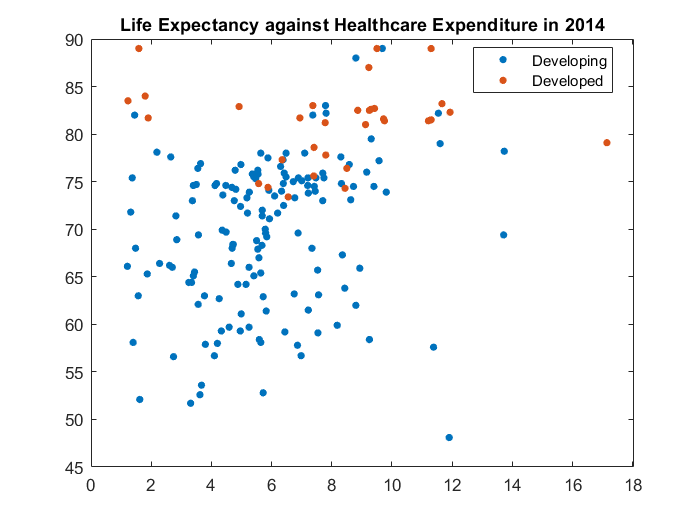
We make 3 observations:
- There are much fewer developed countries (orange) than developing countries (blue).
- Developed countries tend to have higher life expectancy than developing countries.
- Life expectancy MAYBE is positively correlated with heathcare expenditure for developing countries, but less so for developed countries.
Now let’s fit some linear regression models!
We’re going to use the fitlm function in MATLAB. This function provides very detailed outputs.
1
2
3
4
5
6
| data_2014.Status = categorical(data_2014.Status, ["Developing" "Developed"]); %%% note the order
data_2014.LE = data_2014.("Life expectancy");
data_2014.HE = data_2014.("Total expenditure");
m1 = fitlm(data_2014, "LE ~ HE * Status");
% anova(m1, "component", 3) %%% Type III anova
m1 %%% regression coefficients and stats
|
1
2
3
4
5
6
7
8
9
10
11
12
13
14
15
16
17
| m1 =
Linear regression model:
LE ~ 1 + Status*HE
Estimated Coefficients:
Estimate SE tStat pValue
________ _______ _______ __________
(Intercept) 65.288 1.5208 42.93 1.6594e-95
Status_Developed 15.824 3.6356 4.3525 2.2717e-05
HE 0.73836 0.24142 3.0584 0.0025709
Status_Developed:HE -0.73511 0.45121 -1.6292 0.10505
Number of observations: 181, Error degrees of freedom: 177
Root Mean Squared Error: 7.15
R-squared: 0.307, Adjusted R-Squared: 0.295
F-statistic vs. constant model: 26.1, p-value = 5.11e-14
|
Note that it’s critically important to know how to correctly interpret these results, e.g., what is the “Intercept” and whether “HE” is a simple effect or a main effect. See more in Kevin’s post on Interpreting Regression Coefficients. Briefly, the order of the categorical variable AND whether the continuous variable is mean-centered matter. Let’s see:
1
2
3
4
| data_2014.Status_rev = categorical(data_2014.Status, ["Developed" "Developing"]);
data_2014.HE_mc = data_2014.HE - mean(data_2014.HE, "omitmissing");
m2 = fitlm(data_2014, "LE ~ HE_mc * Status");
m3 = fitlm(data_2014, "LE ~ HE_mc * Status_rev");
|
| |
Estimate |
SE |
tStat |
pValue |
| 1 (Intercept) |
65.2878 |
1.5208 |
42.9296 |
0 |
| 2 Status_Developed |
15.8237 |
3.6356 |
4.3525 |
0 |
| 3 HE |
0.7384 |
0.2414 |
3.0584 |
0.0026 |
| 4 Status_Developed:T… |
-0.7351 |
0.4512 |
-1.6292 |
0.1050 |
| |
Estimate |
SE |
tStat |
pValue |
| 1 (Intercept) |
69.8664 |
0.5929 |
117.8317 |
0 |
| 2 Status_Developed |
11.2652 |
1.5557 |
7.2414 |
0 |
| 3 HE_mc |
0.7384 |
0.2414 |
3.0584 |
0.0026 |
| 4 Status_Developed:T… |
-0.7351 |
0.4512 |
-1.6292 |
0.1050 |
| |
Estimate |
SE |
tStat |
pValue |
| 1 (Intercept) |
81.1316 |
1.4382 |
56.4102 |
0 |
| 2 Status_rev_Develop… |
-11.2652 |
1.5557 |
-7.2414 |
0 |
| 3 HE_mc |
0.0032 |
0.3812 |
0.0085 |
0.9932 |
| 4 Status_rev_Develop… |
0.7351 |
0.4512 |
1.6292 |
0.1050 |
Let’s quickly plot the effects of HE (with 95% confidence intervals) on LE, separately for developed and developing countries. This is essentially doing plot(ggemmeans(m, ~ HE + Status)) in R.
1
| plotSlice(m2); %%% alternative syntax: `m2.plotSlice;`
|
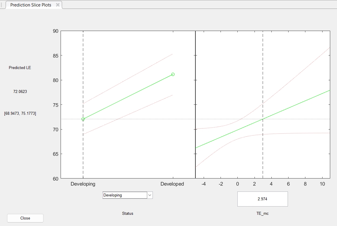
All that looks great! We can now rather confidently report the statistics and make inferences regarding the relationship between life expectancy and health expenditure for developed and developing countries.
However, that was just one regression model. What if we need to fit a much larger number of models, for each of which we don’t really need detailed statistics? We can use the regress function to trade comprehensiveness for speed.
1
2
3
4
5
6
7
8
9
10
| % define outcome variable -- a numeric column vector
y = data_2014.LE;
% define predictor variables -- a numeric array
X = nan(length(y), 4); %%% initialize 4 columns as we have four terms
X(:, 1) = 1; %%% constant term is NOT automatically put into the model!
X(:, 2) = double(data_2014.Status=="Developing"); %%% manually code the categorical variable
X(:, 3) = data_2014.("Total expenditure") - mean(data_2014.("Total expenditure"), "omitmissing");
X(:, 4) = X(:, 2) .* X(:, 3); %%% interaction term
[b, bint, r, rint, stats] = regress(y, X);
b
|
1
2
3
4
5
| b = 4x1
81.1316
-11.2652
0.0032
0.7351
|
Although the regress function does have a stats output, it is actually the statistics regarding the model as a whole (e.g., R-squared and such) rather than individual fixed effects terms. Nevertheless, let’s compare the regression coefficients b from regress to what we obtained from fitlm.
| |
Estimate |
SE |
tStat |
pValue |
| 1 (Intercept) |
81.1316 |
1.4382 |
56.4102 |
0 |
| 2 Status_rev_Develop… |
-11.2652 |
1.5557 |
-7.2414 |
0 |
| 3 HE_mc |
0.0032 |
0.3812 |
0.0085 |
0.9932 |
| 4 Status_rev_Develop… |
0.7351 |
0.4512 |
1.6292 |
0.1050 |
1
| all(m3.Coefficients.Estimate == b)
|
Ta-da! All of the regression coefficients (estimates) are indeed the same! And while we did lose the nice-looking tables filled with statistics, a (very crude) test below shows that regress indeed runs a lot faster than fitlm.
1
2
3
4
5
6
7
8
9
10
11
12
| tic
for i=1:500
y = data_2014.LE;
% define predictor variables
X = nan(length(y), 4); %%% initialize 3 columns
X(:, 1) = 1; %%% constant term is NOT automatically put into the model!
X(:, 2) = double(data_2014.Status=="Developing"); %%% manually code the categorical variable
X(:, 3) = data_2014.("Total expenditure") - mean(data_2014.("Total expenditure"), "omitmissing");
X(:, 4) = X(:, 2) .* X(:, 3); %%% interaction term
[b, bint, r, rint, stats] = regress(y, X);
end
toc
|
1
| Elapsed time is 0.201044 seconds.
|
1
2
3
4
5
| tic
for i=1:500
m = fitlm(data_2014, "LE ~ HE_mc * Status_rev");
end
toc
|
1
| Elapsed time is 5.250400 seconds.
|
5. Conclusion
We’ve made it to the end of MATLAB basics and regression (yay!), though this is just the tip of the iceberge of regression models out in the wild world, such as regularized regression, nonlinear regression, and mixed-effects regression. Feel free to check out how they are can be implemented in MATLAB here.

Enjoying MATLAB-ing!